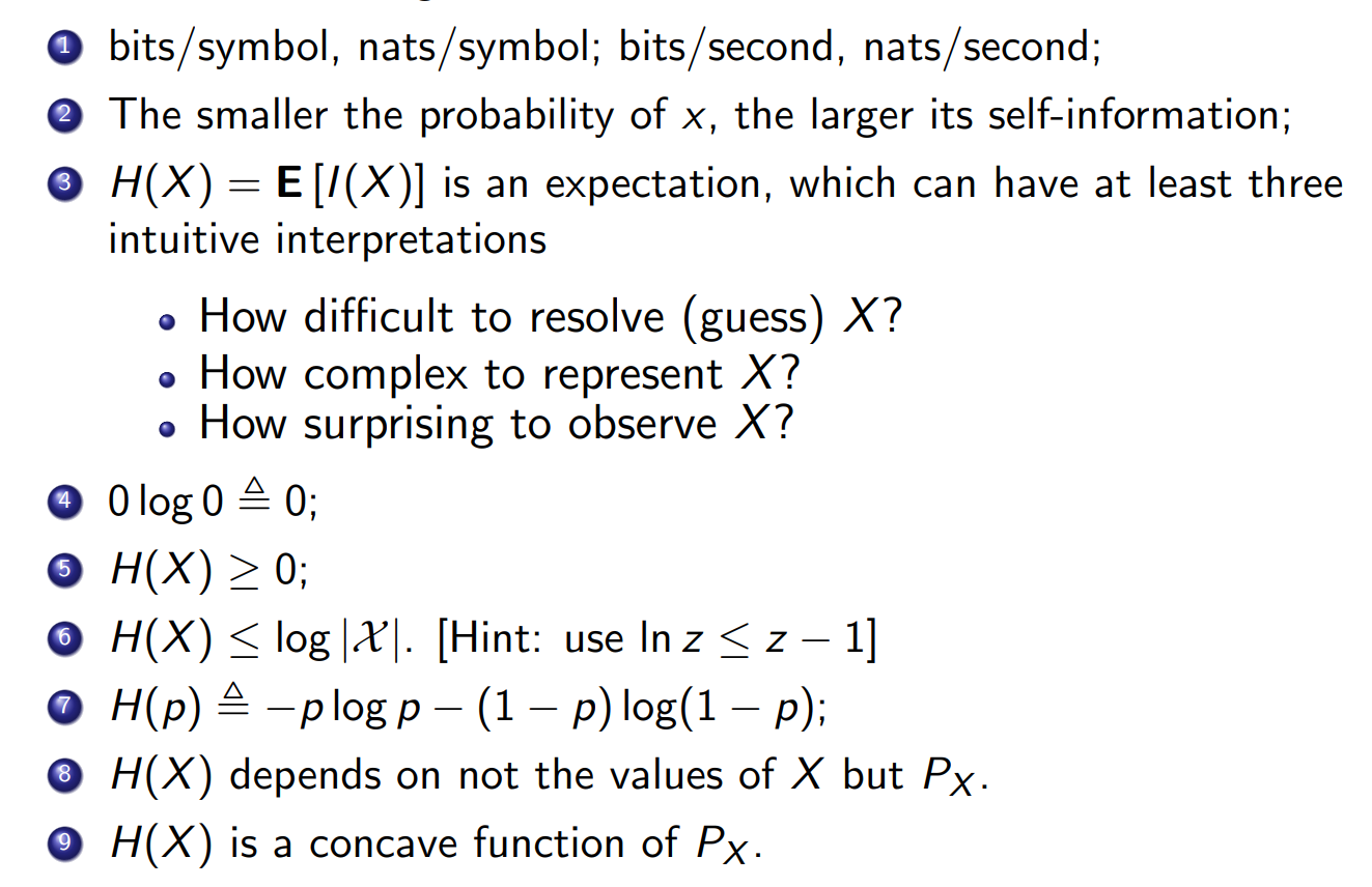
Self -information
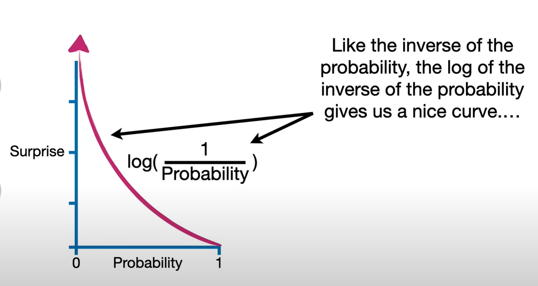
In information theory and statistics, “surprise” is quantified by self-information. For an event x with probability p(x), the amount of surprise (also called information content) is defined as
This definition has several nice properties:
Rarity gives more surprise: If p(x) is small, then I(x) is large — rare events are more surprising.
Certainty gives no surprise: If p(x)=1, then I(x)=0. Something guaranteed to happen is not surprising at all.
Additivity for independence: If two independent events occur, the total surprise is the sum of their individual surprises: I(x,y)=I(x)+I(y)
The logarithm base just changes the unit:base 2 gives “bits,” base e gives “nats.”
For example, if an event has probability 1/8, then
meaning the event carries 3 bits of surprise.
Entropy
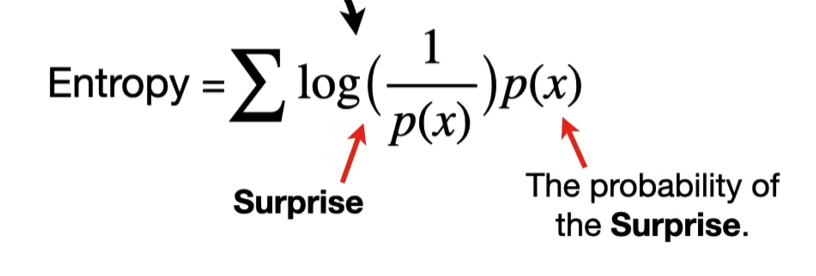
Formally, entropy is defined as the expected surprise (expected self-information) under a probability distribution. For a random variable X with distribution p(x):
Key points:
Each outcome x carries a “surprise”
. We weight that surprise by how likely it is p(x).
The entropy is the average surprise if you repeatedly observe X.
For example:
A fair coin (
) has Meaning: on average, each coin flip carries 1 bit of surprise.
A biased coin (
) has Less uncertainty → less average surprise.
So entropy = expected surprised amount you’d feel per observation, given your model.
Entropy (general concept)
Entropy is a property of a random variable.
If X is a discrete random variable with distribution p(x), then:
So here, H(X) means “the entropy of random variable X.”
H(p)(entropy as a function of a distribution)
Instead of thinking of entropy as tied to a random variable, we can think of it as a function of the probability vector p:
This view treats entropy as a mathematical function on the simplex of probability distributions.
It’s in this sense that we say “H(p) is concave in p.”
Cross-entropy
The weighting comes from the true distribution P (because that’s what actually happens in the world).
The surprise calculation
comes from the model Q (because that’s what you believe the probabilities are). Reality probability P:
In theory: it’s the true distribution of the world.
In practice: we don’t know it exactly, so we estimate it from data (observations, frequencies, empirical distribution).
Example: if in 100 flips you saw 80 heads and 20 tails, then your empirical P is 0.8 ,0.2.
Model probability Q:
This is your hypothesis or predictive model.
It gives probabilities for outcomes (e.g. “I think the coin is fair, so Q=0.5,0.5”).
It can be parametric (like logistic regression, neural network, etc.) or non-parametric.
Property of source information
i.i.d. (independent and identically distributed) is a special case of “memoryless + stationary,” but the concepts are slightly different.
i.i.d. is a property of the information source — a sequence of random variables
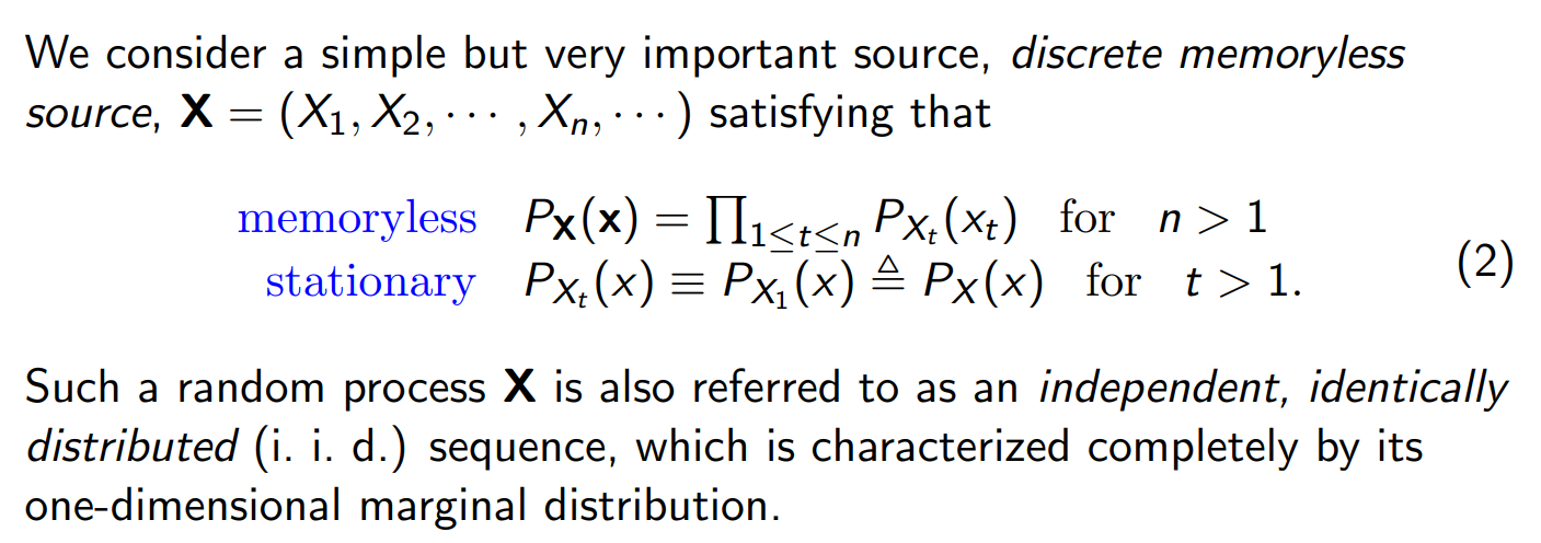
Stationary
Means the distribution is the same over time.
Example:
for all t. Does not require independence.
You could have correlations (like a Markov chain) and still be stationary if the distribution doesn’t change with time.
Memoryless
Means no dependence on the past (i.e. independence).
Example:
Does not require the distribution to be identical over time. (E.g. each toss independent but the bias slowly changes with time → memoryless but not stationary.)
i.i.d.
Independent: no memory (memoryless).
Identically distributed: stationary in the simplest sense (same marginal distribution for all time steps).
So i.i.d. = memoryless and stationary at once.
Joint entropy
For two random variables
Interpretation: the average surprise when you observe the pair
- If X and Y are independent:
Conditional entropy
The conditional entropy of Y given X is
🔹 Interpretation: the average surprise in Y after you already know X.
If X and Y are independent:
If Y is fully determined by X:
Definition of conditional entropy
But
So
Intuition
Conditional entropy measures the remaining uncertainty in one variable after knowing another.
If you condition on the same variable, there is no uncertainty left at all.
Therefore:
Chain rule of entropy
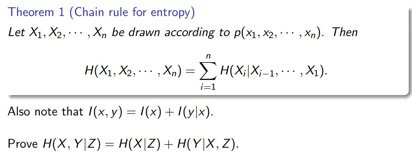
For two random variables X and Y
This is called the chain rule for entropy.
Why it works
Start from the definition of joint entropy:
Factorize p(x,y):
So:
Expand the log:
The first term simplifies to
The second term is exactly H(Y∣X).
to a simpler result. Let’s work it step by step.
Factor the sums
Recognize conditional distribution
Note that
So:
The inner sum
is just the entropy of Y given a fixed X=x. Call this
So the whole expression becomes:
Symmetry
By symmetry, you can also write
Chain rule without conditioning
This is the basic chain rule of entropy.
It says: the uncertainty in the pair (X,Y) equals the uncertainty in X plus the leftover uncertainty in Y once you know X.
No external variable here.
In general case:
Chain rule with conditioning on Z
This is the conditional chain rule.
It says: given knowledge of Z, the uncertainty in the pair (X,Y) equals:
the uncertainty in X once you know Z, plus
the leftover uncertainty in Y once you know both X and Z.
out the uncertainty of (X,Y)once Z is already given.
In general case:
Conditioning reduces entropy
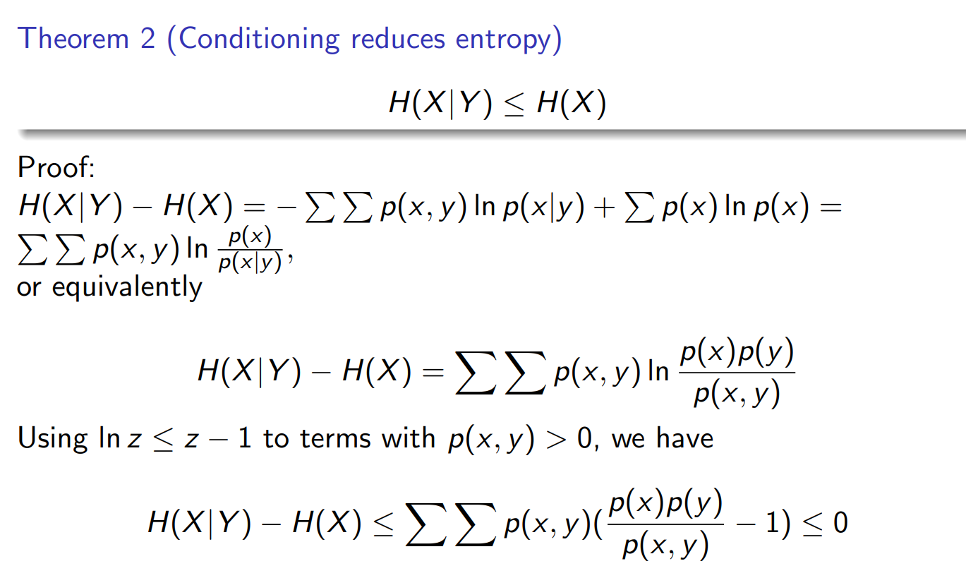
The intuition behind the inequality
comes from the “surprise” perspective in information theory. Entropy measures the average surprise you get when observing outcomes.
Entropy H(X): This is the average surprise of seeing X when you don’t know anything else.
Conditional entropy H(X∣Y): This is the average surprise of seeing X when you already know Y.
Now, knowing more information (conditioning on Y) can only reduce your uncertainty about X—or at worst, leave it unchanged. Think of “surprise” like how much a new observation catches you off guard: if I already tell you some side information Y, you’re usually less surprised when you see the actual X, because you had a better guess in advance. That’s why H(X∣Y)can never exceed H(X).
H(p) is a concave function of probability
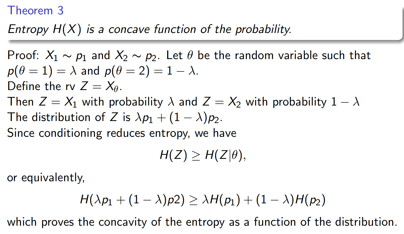
More precise:
You have two candidate random variables:
Then you toss
: If
, you set . If
, you set .
So Z equals one of the two random variables, chosen according to
Example (mixture of coins):
: coin with Pr(H)=0.2, Pr(T)=0.8 : coin with Pr(H)=0.9, Pr(T)=0.1. θ∼Bernoulli(λ=0.5).
Then:
If θ=1, Z is distributed like
. If
, Z is distributed like Overall, the distribution of Z is the mixture:
Take the simplest case: a binary random variable with probabilities
Entropy is
This function
is concave in p. Concavity means: for any two probability values
and any
Graphically, the entropy curve is shaped like an “upside-down bowl.”
Maximum at
(most uncertainty). Minimum at
or (no uncertainty).
This concavity holds more generally: entropy is concave in the whole probability distribution p(x) .
That’s why mixing distributions increases entropy (on average).
Kullback-Leibler distance
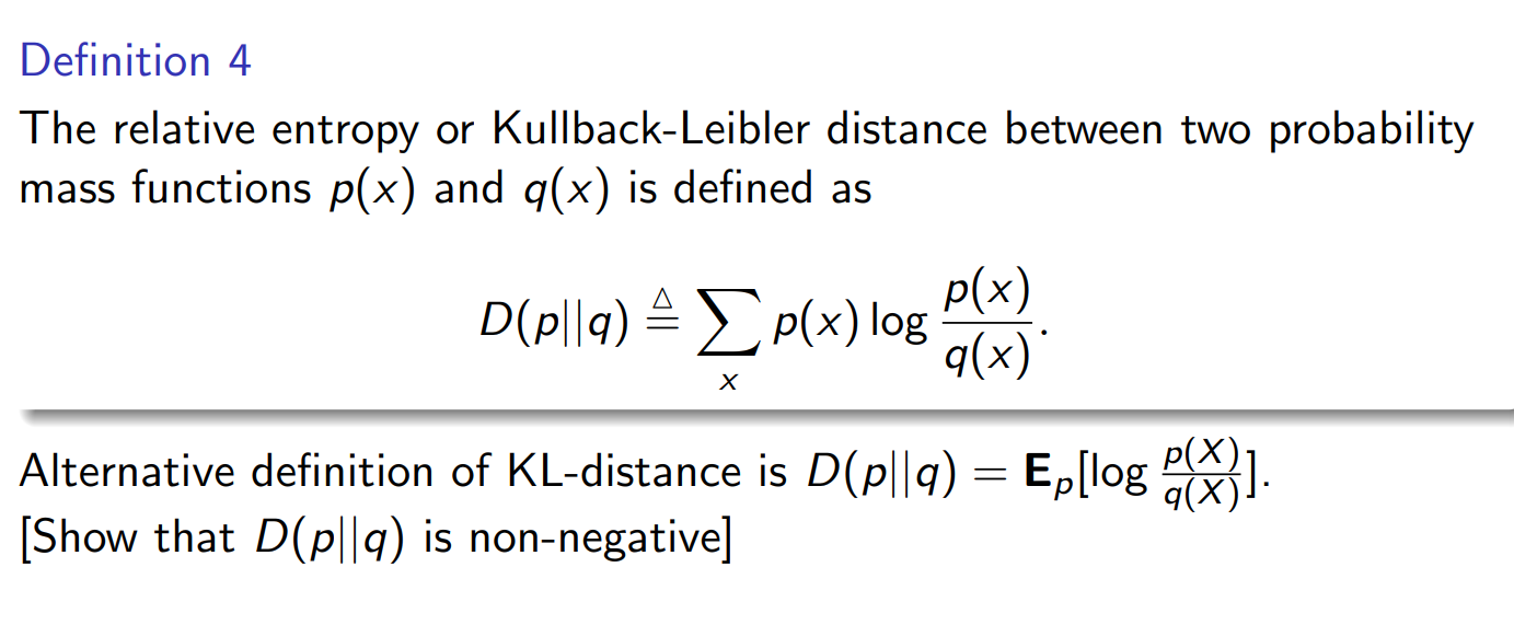
D(p∥q) is the extra surprise (expected log-likelihood ratio) when you think data comes from q but it actually comes from p.
It measures how much information you lose if you approximate p by q.
Entropy H(p): your true average surprise if you use the correct distribution.
Cross-entropy H(p,q): your average surprise if you believe the world is q but reality is p.
KL divergence: the extra surprise (or inefficiency) caused by using the wrong distribution q instead of the true one p.
p(x) = true distribution (nature, or the data-generating process).
q(x) = model/hypothesis you assume.
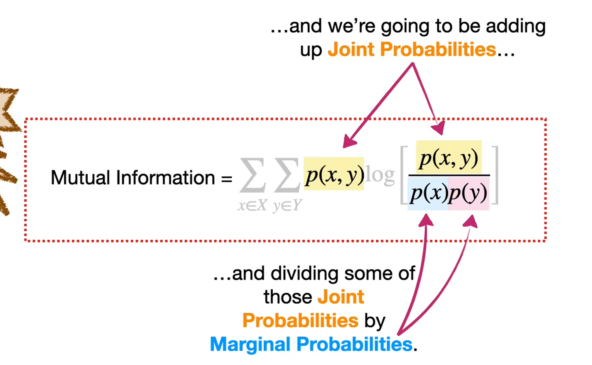
Mutual Information
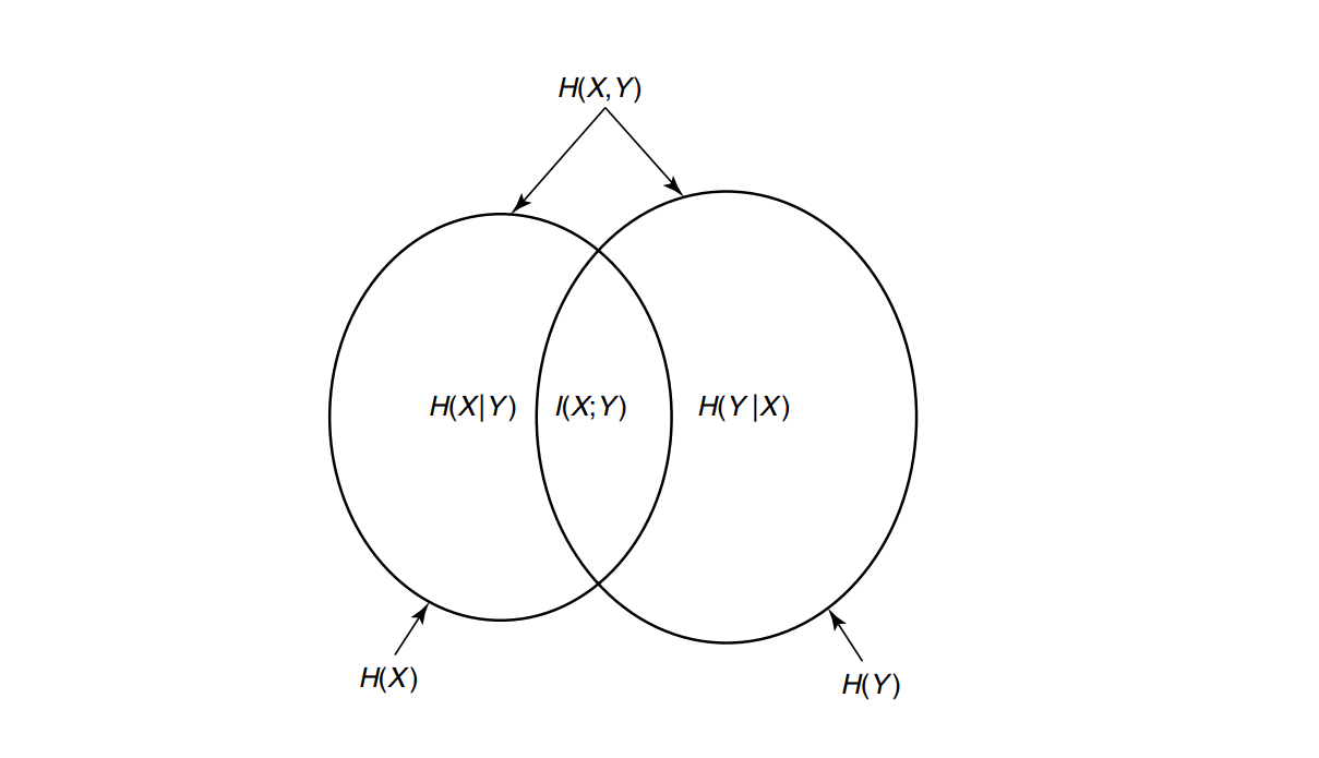
The mutual information between two random variables X and Y is
It can also be written as
And in terms of distributions:
shows the symmetry: it’s also the reduction in uncertainty about Y when you know X.
That’s why we say mutual information is the common information (or “shared surprise”) between X and Y.
Mutual Information as a measure of dependence
If I(X;Y)=0: the two variables are independent. Knowing one tells you nothing about the other.
If I(X;Y) is large: there is a strong dependency. Knowing one variable reduces a lot of uncertainty about the other.
How “large” relates to entropy
The maximum possible mutual information is limited by the entropy:
This makes sense: you can’t learn more about Y from X than the total uncertainty H(Y) that Y has.
Intuition with examples
Independent coin flips:
. Perfect correlation (e.g. Y=X):
Perfect anti-correlation (e.g.
):
as well — because knowing one still completely determines the other.
So yes, larger MI = stronger relationship between the two variables.
Chain rule of mutual inforamtion
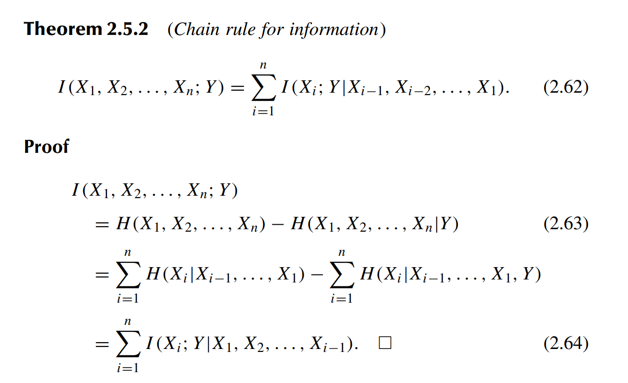
The statement
This says:
The total information that all variables
Why is this true?
Start from the definition:
Now apply the entropy chain rule:
Subtracting gives:
But each bracket is exactly:
So the theorem follows.
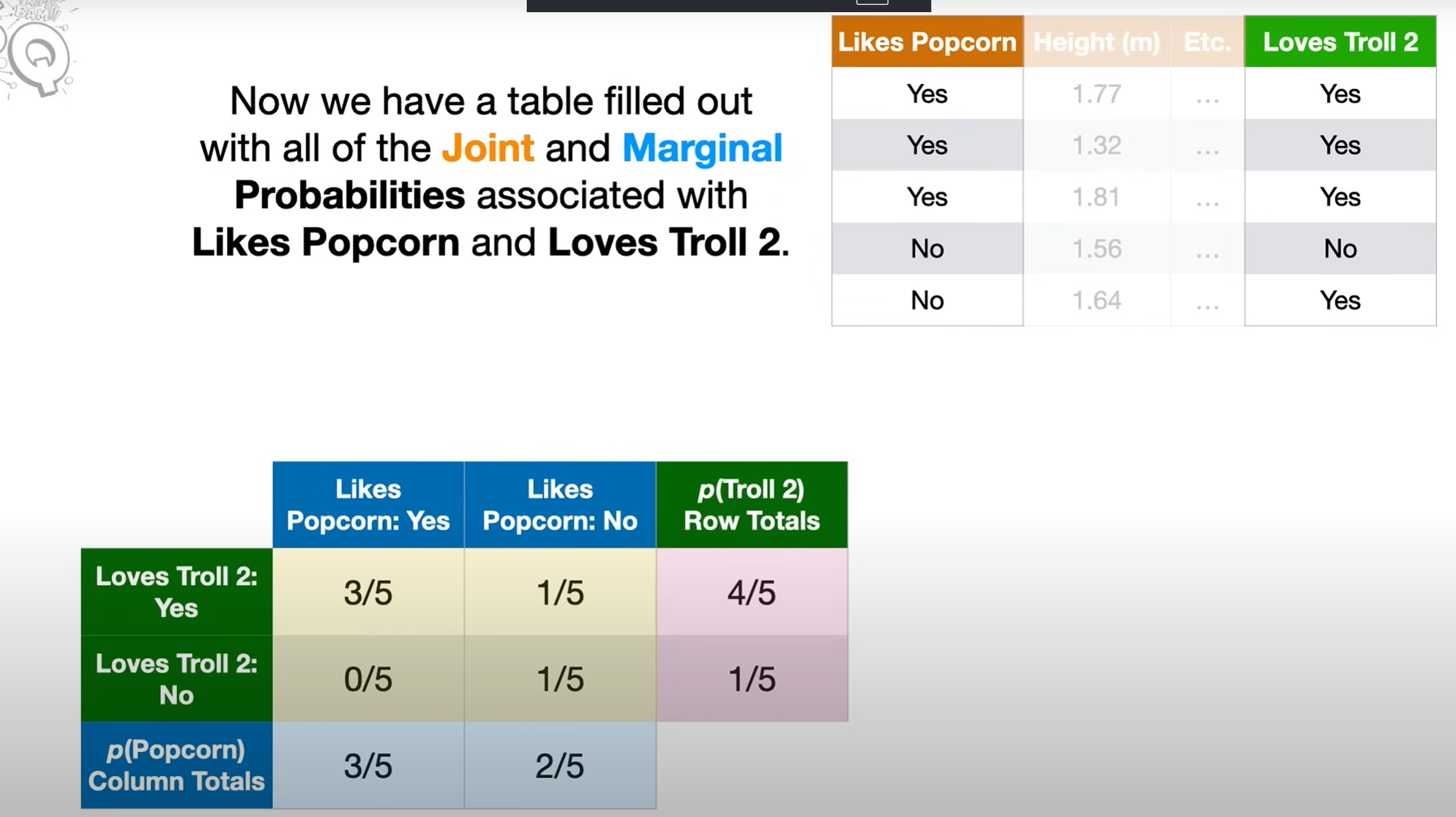
Marginal probability
- Marginal” means you’re looking at the distribution of one variable alone, ignoring the others.
- On a probability table, you literally get it by summing along the margins — that’s why it’s called marginal probability.