What is information theory and coding

goal

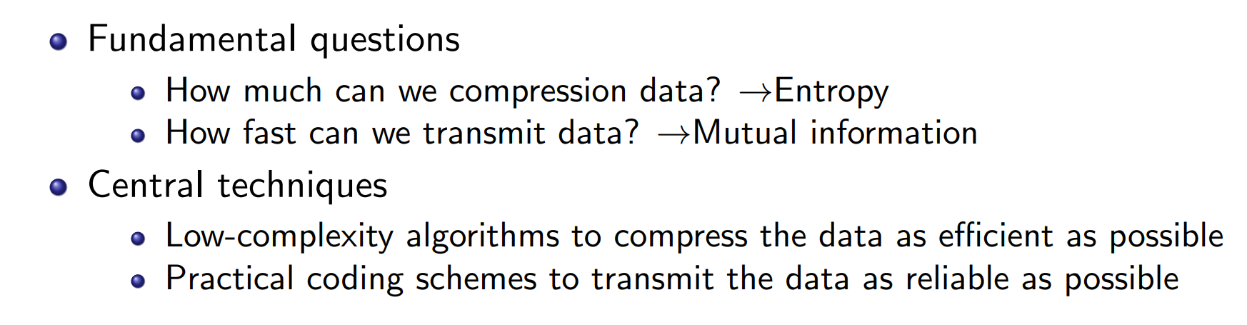
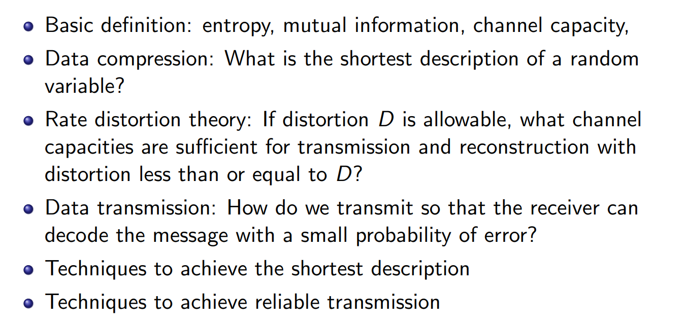
what should we learn

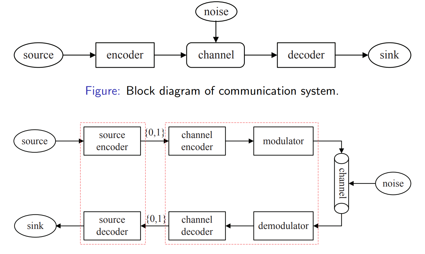
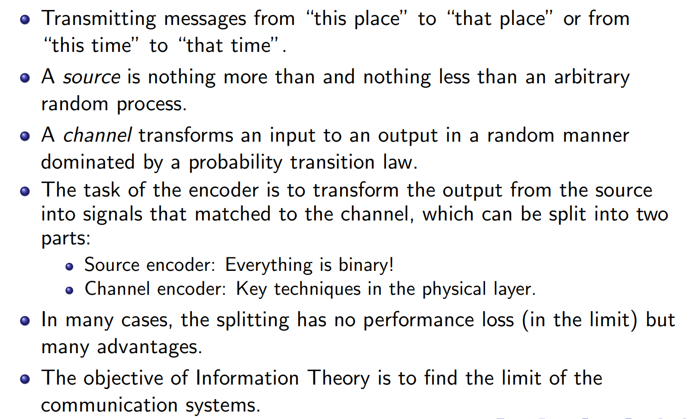
communication system

• Source Encoder

  • Converts the raw source (text, audio, image) into a sequence of bits .

• Channel Encoder

  • Adds redundancy to protect against noise.

• Modulator

  • Converts the encoded bits into waveforms/signals that can physically travel through the channel.

• Channel + Noise

  • The medium distorts the signal (attenuation, interference, random noise).

• Demodulator

  • Recovers the bit sequence from the noisy received signal.

• Channel Decoder

  • Uses redundancy added earlier to detect and correct errors.

• Source Decoder

  • Reconstructs the original message from the bit sequence (decompression, translation back to human-readable form).

• Sink

  • The final destination (e.g., your ear for audio, your screen for video, or your computer program).

Encoder

• Works at the information/coding level (bit sequences).

• Two main types:

  • Source encoder: compresses data into binary (e.g., JPEG, MP3, Huffman coding).

  • Channel encoder: adds redundancy for error protection (e.g., Hamming code, LDPC, Turbo codes).

• Input/output:

  • Takes raw data → outputs a stream of bits {0,1}{0,1}.

• Purpose: make data efficient and reliable before physical transmission.

Modulator

• Works at the signal/physical layer.

• Converts the encoded bitstream into waveforms that can be transmitted over the physical medium (radio waves, optical fiber, etc.).

• Examples:

  • BPSK (binary phase shift keying)

  • QAM (quadrature amplitude modulation)

  • OFDM (used in WiFi, 4G/5G)

• Input/output:

  • Takes binary bits → outputs analog/electromagnetic signals.

• Purpose: adapt binary data to the physical channel so that it can actually travel.

information

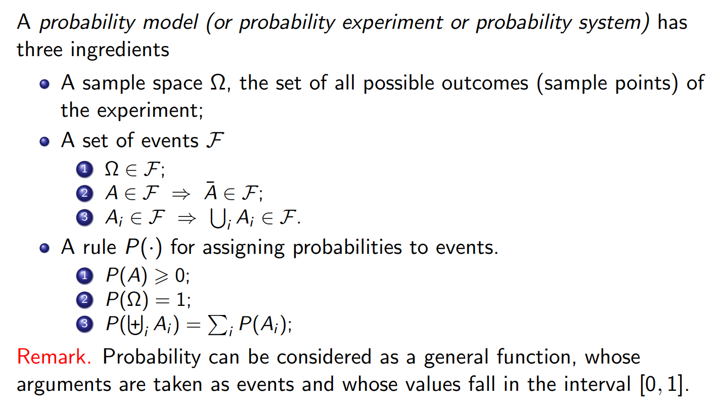
Probability Model

Probability law

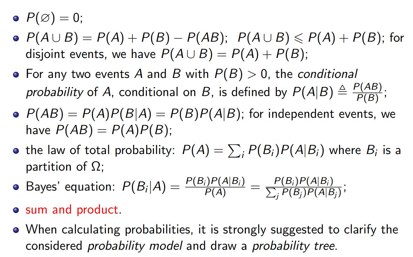
Bayes’ equation

The Formula

Bayes’ theorem relates conditional probabilities:

where:

• P(A) = prior probability of event A.

• P(B∣A) = likelihood of observing B given A.

• P(B) = total probability of B (normalizing factor), computed as

if are all possible hypotheses.

Interpretation

• Prior P(A): what you believed before seeing data.

• Likelihood P(B∣A): how compatible the data is with your hypothesis.

• Posterior P(A∣B): your updated belief after seeing the data.

Random Variable

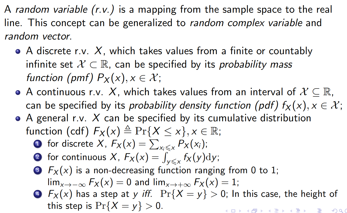
Relationship Between X and

• The random variable X is the mapping from outcomes to numbers.

• The PMF is the distribution that tells us how likely each number is.

• X = “what values are possible?” (e.g. 1–6 for a die).

• ​ = “how are probabilities spread across those values?” (e.g. each has probability 1/6).

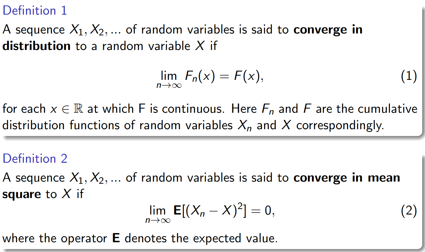
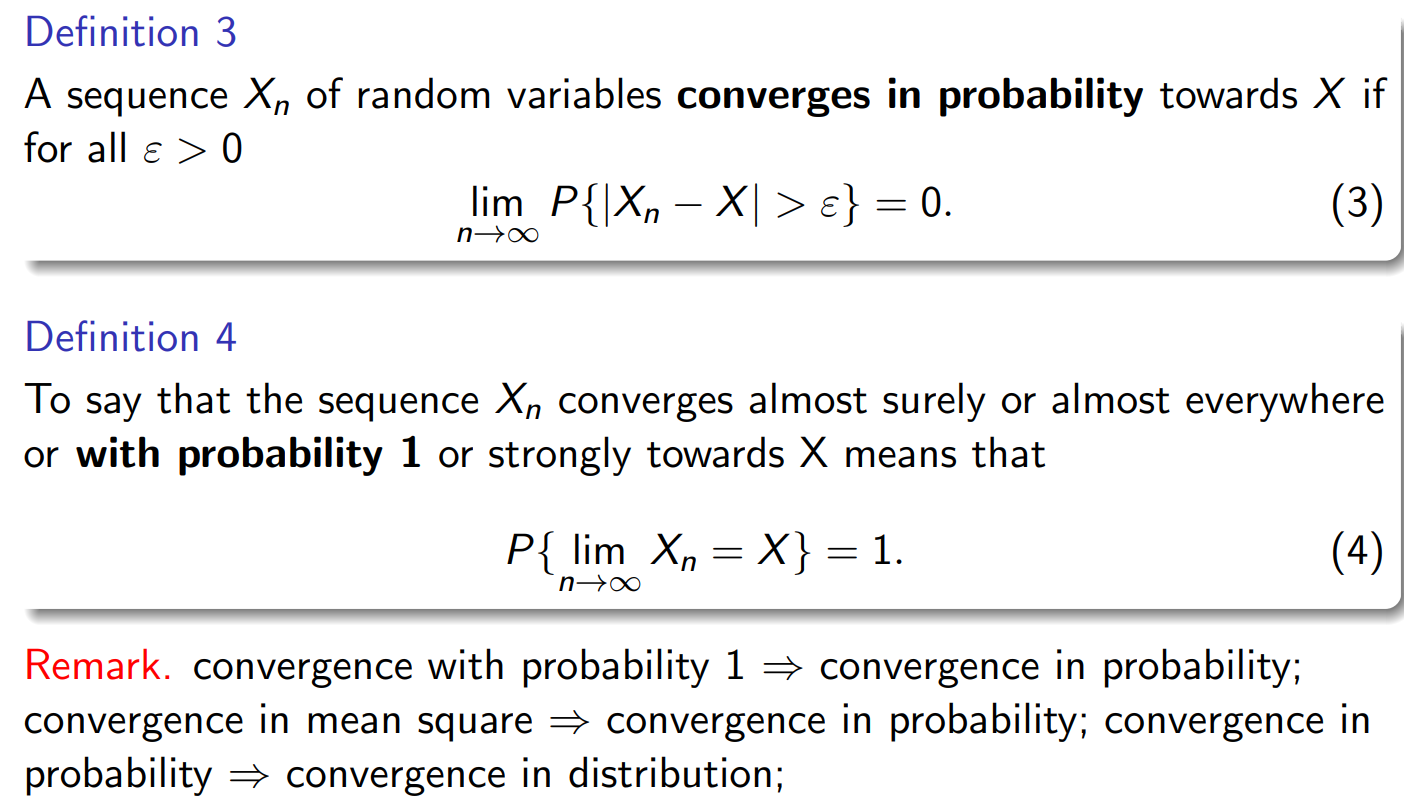
Convergence