
Least squares prediction
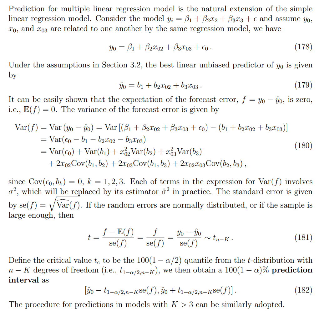
CI and PI
CI: “Where is the average wage for people with 16 years of education likely to be?”
PI: “If I pick one random person with 16 years of education, what wage will they likely earn?”
Confidence Interval (CI)
Target: The conditional mean
This is a fixed but unknown number (not random once the data and
are fixed). The randomness comes from the estimation process (sampling variation in
). So the CI is telling you: “With 95% confidence, the true mean lies in this range.”
CI → fixed but unknown parameter (deterministic).
Prediction Interval (PI)
Target: A new observation
Even if you knew the regression line exactly, this
would still be random because of the error term ε\varepsilonε. PI accounts for both the estimation uncertainty and the irreducible randomness.
So PI is telling you: “With 95% probability, the next individual value will fall in this range.”
PI → random variable (future realization of
).
Summary
CI → fixed but unknown mean, interval comes from the randomness of the estimator.
PI → inherently random individual outcome, interval accounts for both estimation error and noise
Indicator Variables
dummy variables
They are also called dummy, binary, or dichotomous variables, because they take just two values, usually one or zero, to indicate the presence or absence of a characteristic or to indicate whether a condition is true or false. For variables that take on only two values, the mapping to {0, 1} is very common. However other numerical values can also be adopted.
For example, we can define an indicator variable
	D    • D = 1 if characteristic is present;

		• D = 0 if characteristic is not present.
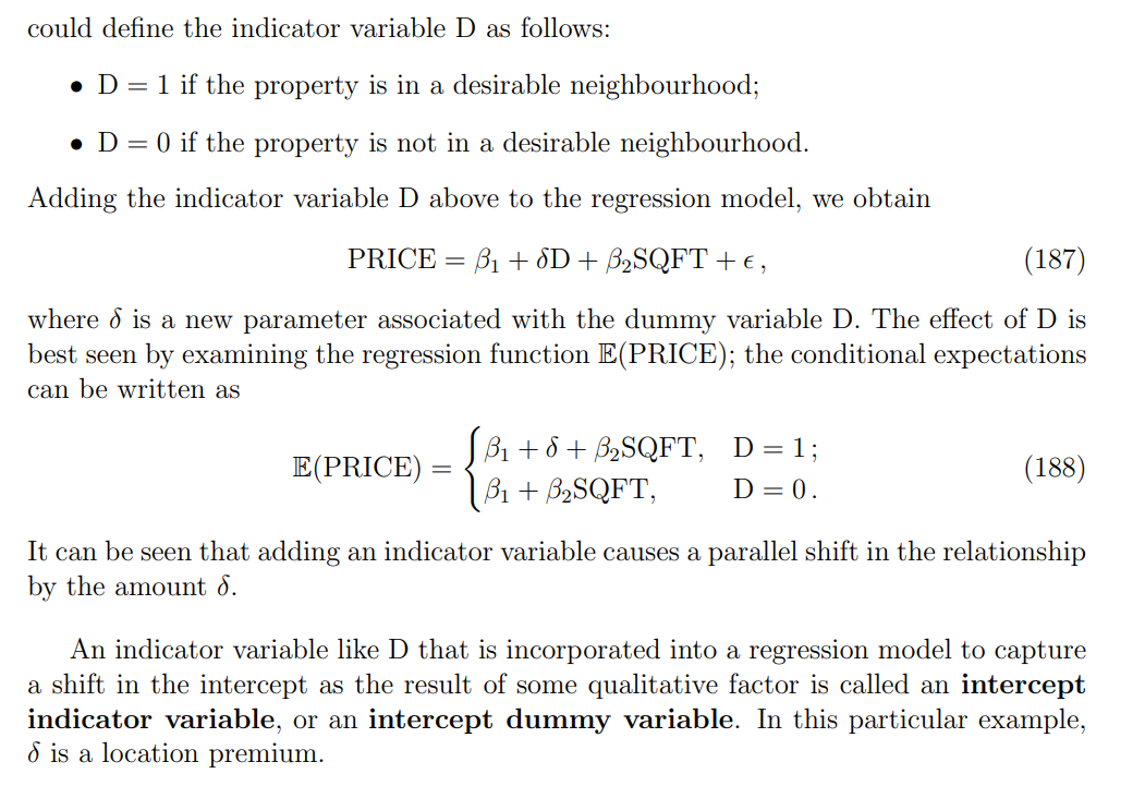
Intercept indicator variables
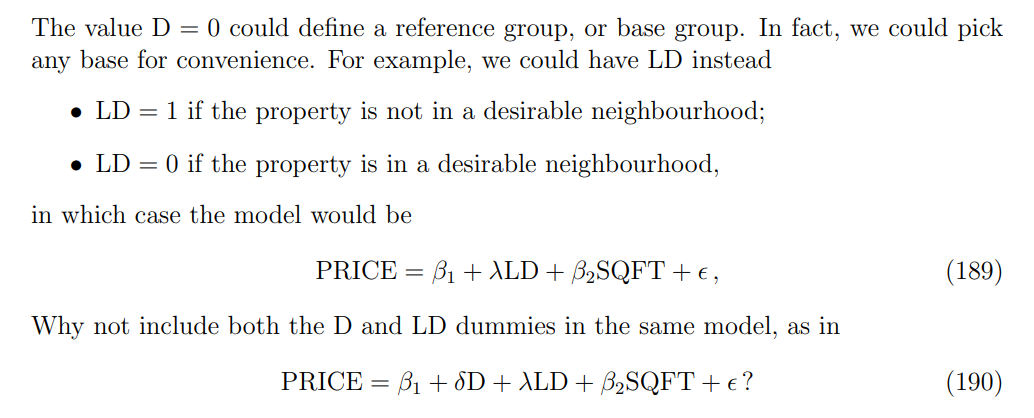
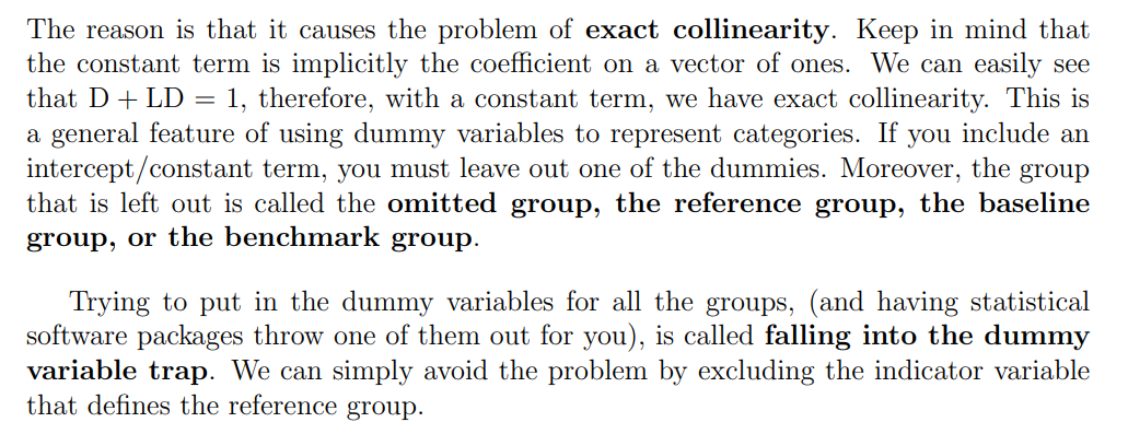
The reference group and the dummy variable trap
Slope indicator variables
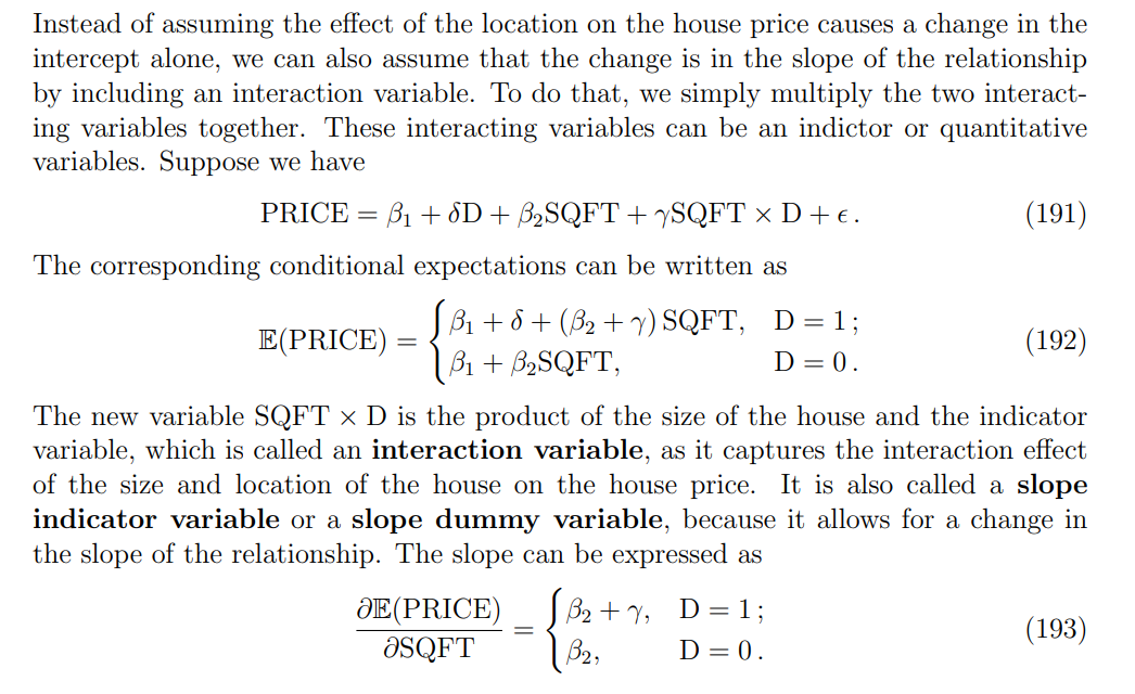
Interactions between qualitative factors
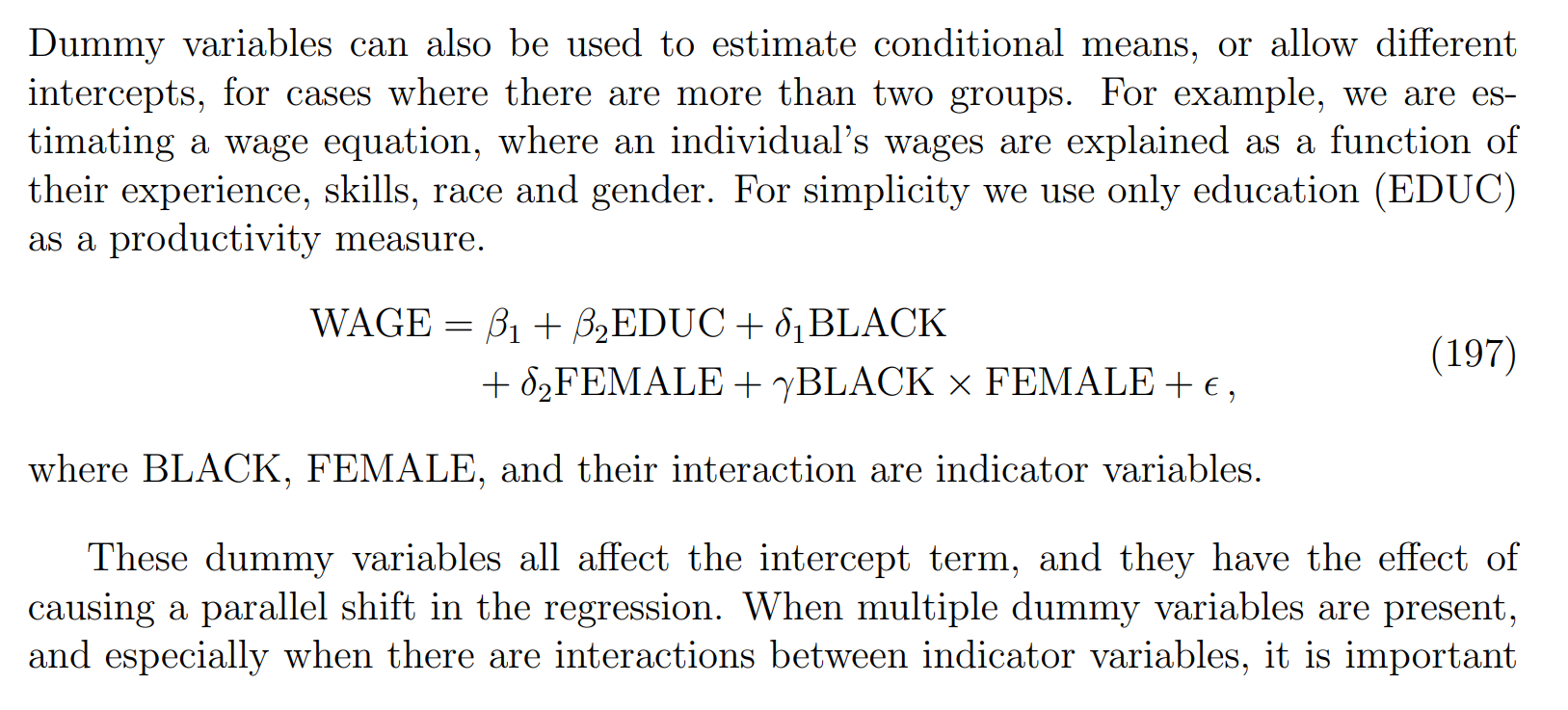
Why do we need an extra coefficient (
) for the interaction between being Black and Female, instead of just letting the two dummy variables (Black, Female) both equal 1?
Two dummy variables only (no interaction term)
Suppose the regression is:
If someone is Black Female, then BLACK=1,FEMALE=1
Their expected wage would be:
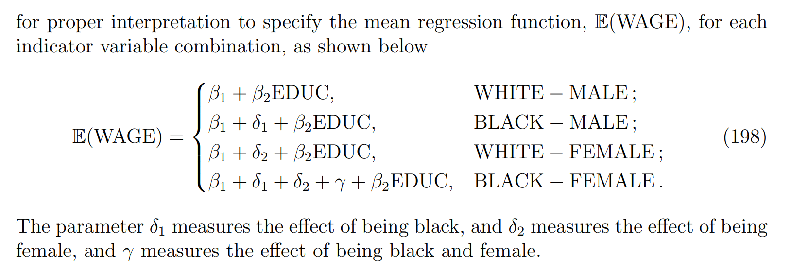
So in this model, the effect of being Black and Female is just the sum of the two separate penalties.
With an interaction term
Now suppose the model is:
If someone is Black Female, then BLACK=1, FEMALE=1, so the interaction term = 1.
Their expected wage is:
Here,
Here,
Why no perfect collinearity?
The interaction column is not equal to either BLACK or FEMALE.
And it’s also not equal to their sum or difference.
It is only “1” in one cell (Black Female), “0” elsewhere.
So mathematically:
for any constants a,b,c
Thus, the interaction term provides new independent information and does not cause perfect collinearity.