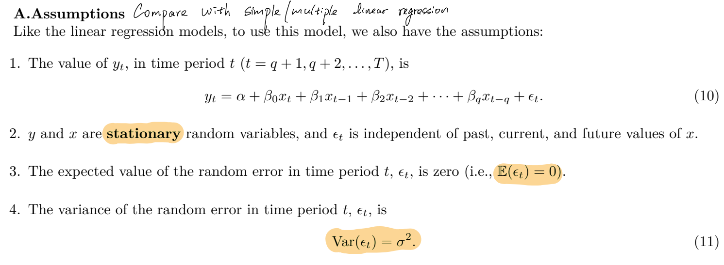
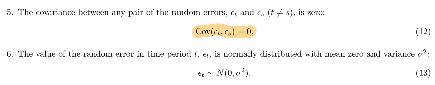
Assumption of linear model
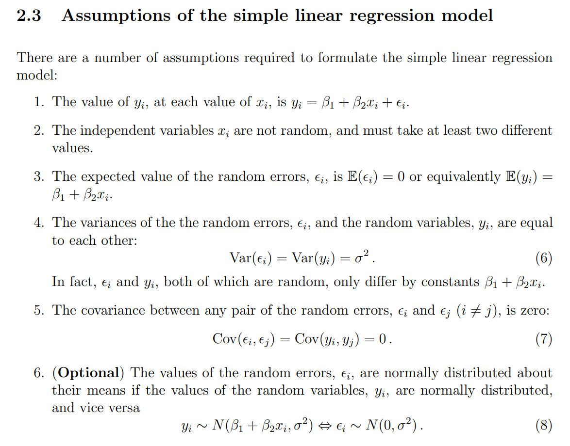
The simple linear regression model is based on the following assumptions.
(i)
(ii) The regressor
(iii)
(iv)
(v)
(vi) (Optional)
第二点解析:
解释变量(自变量)非随机性:
假设是固定的常数,而不是随机变量(即所谓的 fixed in repeated samples)。这样做的好处是,推导估计量的分布时只需要考虑误差项 的随机性,避免了 自身的不确定性带来的额外复杂性。 解释变量必须有变动性:
至少要有两个不同的取值,否则所有 都相同,回归模型退化为 ,根本无法估计斜率 。换句话说, 必须有非零方差,才能保证回归矩阵可逆,估计量 才能被唯一确定。
不需要 6 点都满足才能用(OLS)
真正必须的只有前 1–5 点(高斯–马尔可夫条件)。
第 6 点(误差项正态分布)不是必须条件,它只在你要做:
t 检验
F 检验
构造置信区间
才进一步假设。
least square estimate
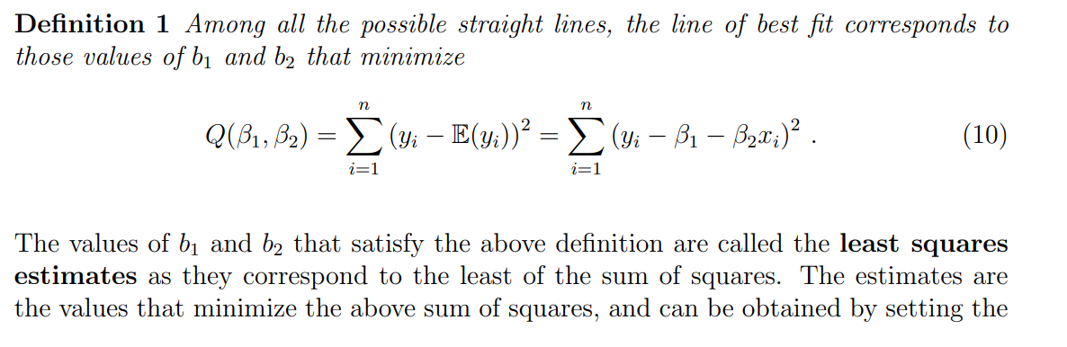
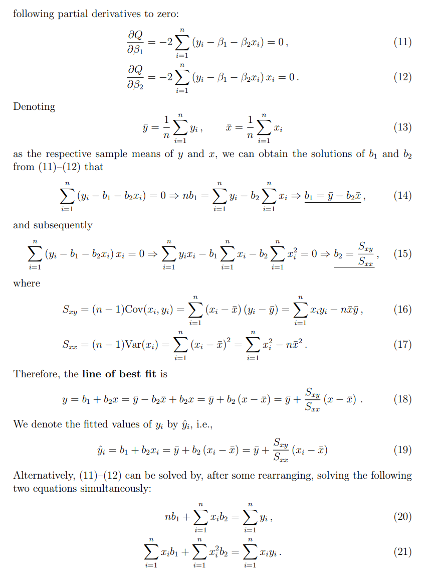
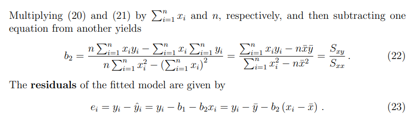
注意:写完
b是怎么求解的。
例题
由于,这些方程等价于:
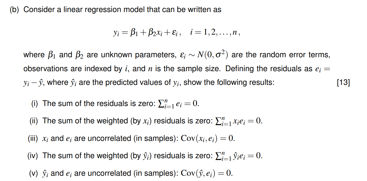
下面分别证明各部分。
(iii) 证明
样本协方差定义为:
由 (i) 知
展开求和:
由 (ii) 和 (i) 知
因此,
(iv) 证明
由于
$$\sum_{i=1}^n \hat{y}i e_i = \sum{i=1}^n (\hat{\beta}_1 + \hat{\beta}_2 x_i) e_i = \hat{\beta}1 \sum{i=1}^n e_i + \hat{\beta}2 \sum{i=1}^n x_i e_i$$
由 (i) 和 (ii) 知
因此,加权残差之和为零。
**(v) 证明 **
样本协方差定义为:
$$\text{Cov}(\hat{y}i, e_i) = \frac{1}{n} \sum{i=1}^n (\hat{y}_i - \bar{\hat{y}})(e_i - \bar{e})$$
由 (i) 知
$$\text{Cov}(\hat{y}i, e_i) = \frac{1}{n} \sum{i=1}^n (\hat{y}_i - \bar{\hat{y}}) e_i$$
展开求和:
$$\sum_{i=1}^n (\hat{y}i - \bar{\hat{y}}) e_i = \sum{i=1}^n \hat{y}i e_i - \bar{\hat{y}} \sum{i=1}^n e_i$$
由 (iv) 知
因此,
Gauss-Markov thm
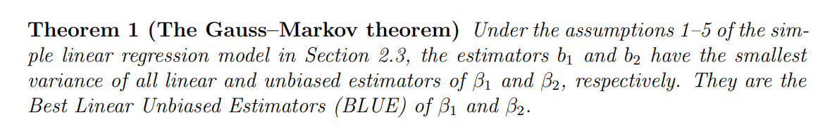
Gauss–Markov 定理内容:在经典线性回归假设下(线性模型、误差期望为零、误差方差相同且有限、误差不相关),最小二乘估计量
换句话说,
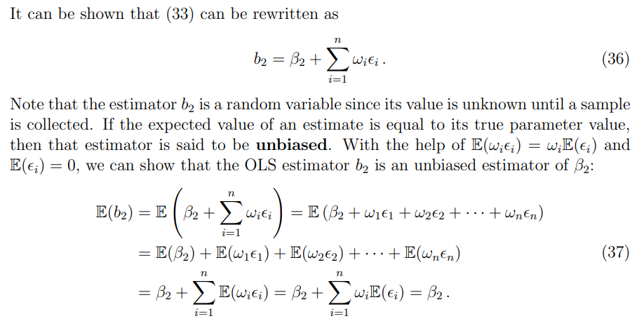
estimator
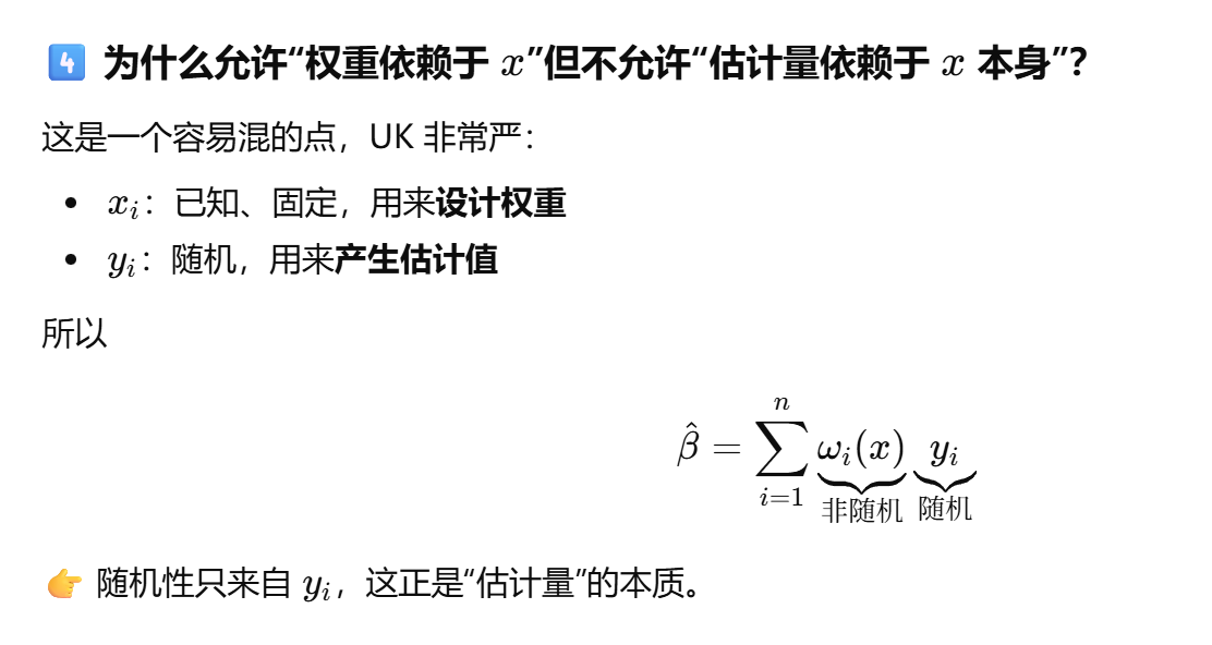
只有在把估计量“代回真实数据生成过程(DGP)”时,才会显式引入真实参数
linear
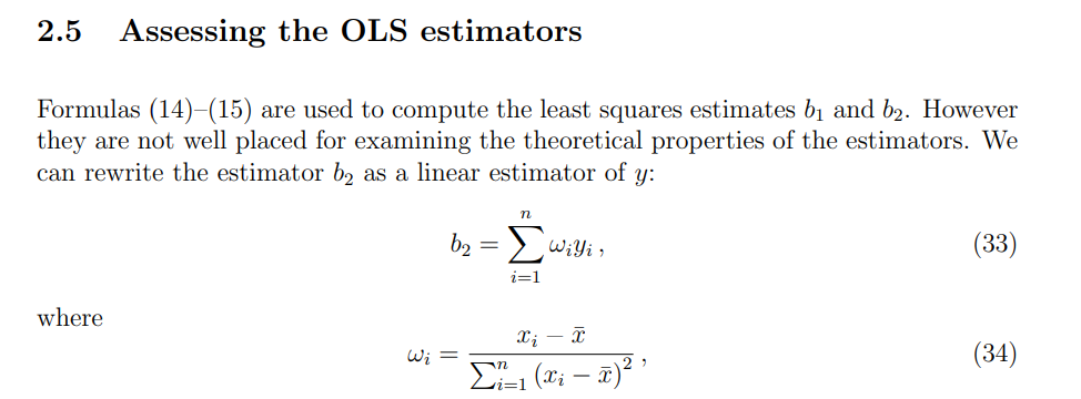
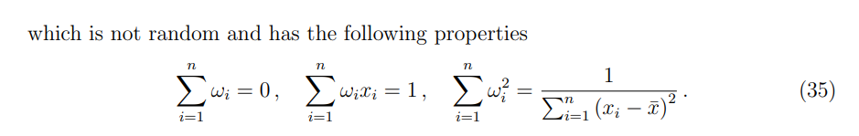
unbiased
MSE(均方误差)
The mean squared error (MSE):
例题:
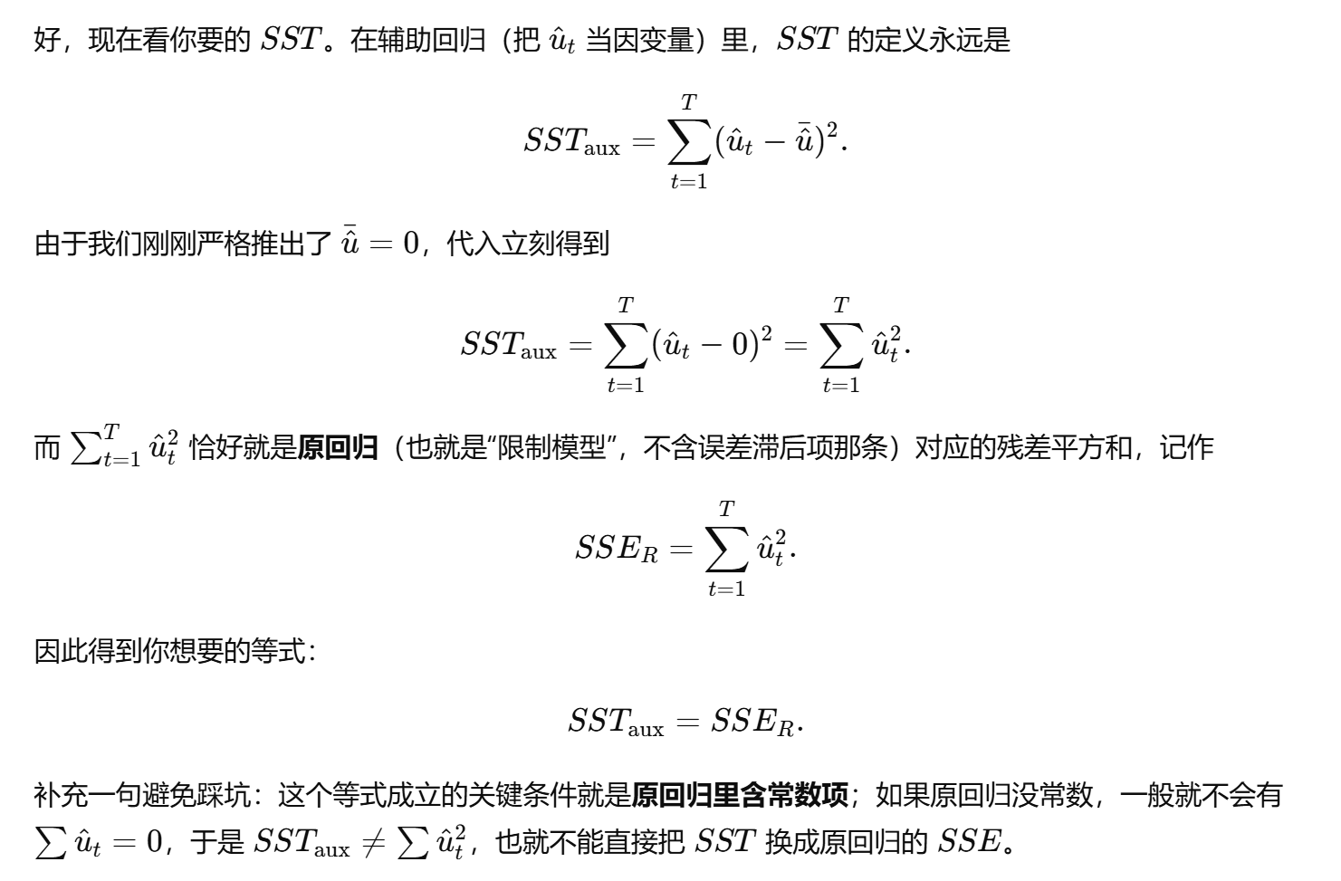
SST
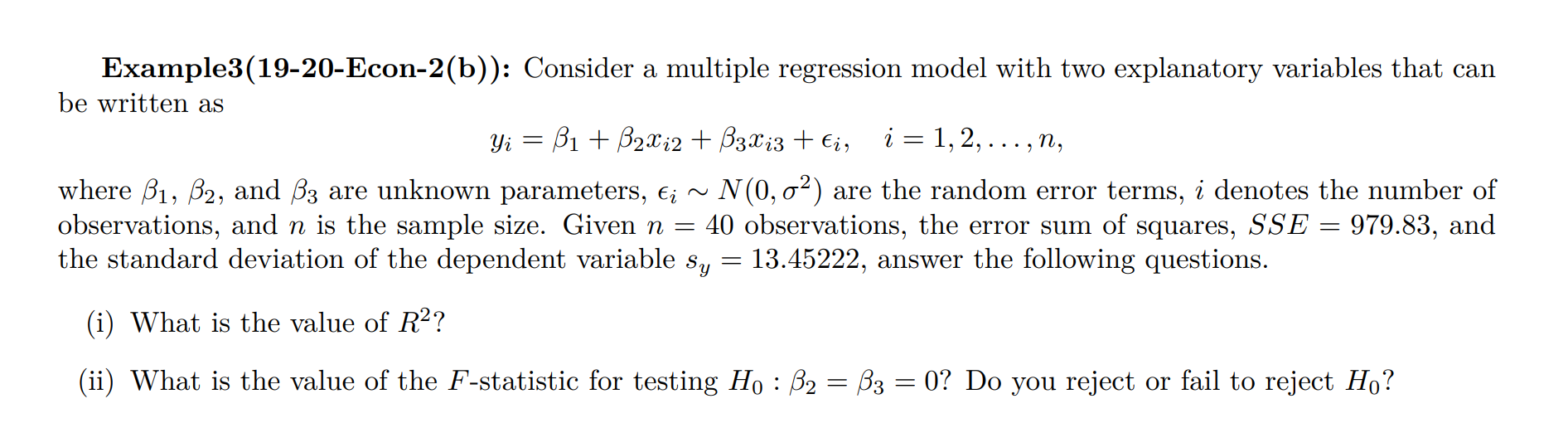
$SST=∑{i=1}^n(y{i}−\bar{y})^2=(n−1)s_{y}^2$
Coefficient of determination(SST=SSR+SSE)
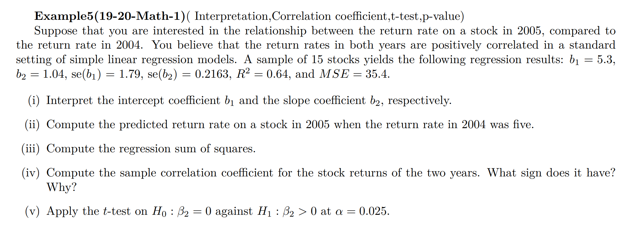
correlation coefficient

例题
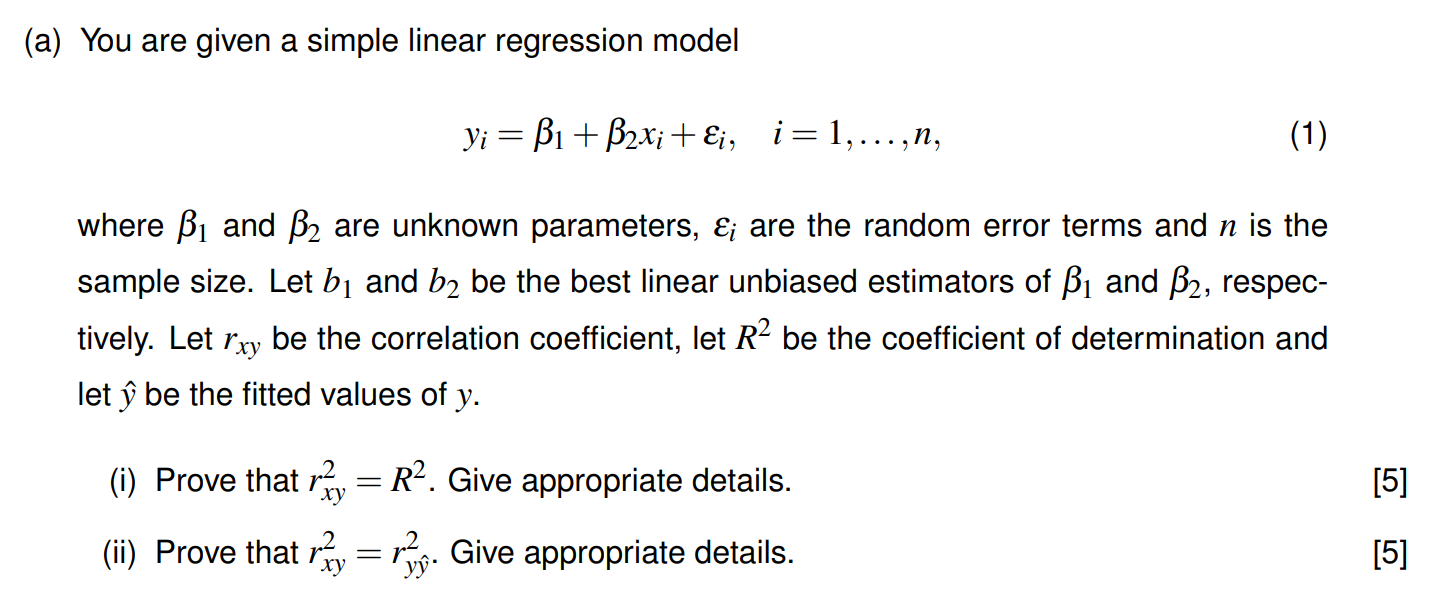
Solution
(i) Prove that
The correlation coefficient
Thus,
The coefficient of determination
where $SSR = \sum_{i=1}^n (\hat{y}i - \bar{y})^2
The OLS estimator
Since the regression line passes through the point
Therefore,
$$SSR = \sum_{i=1}^n (\hat{y}i - \bar{y})^2 = b_2^2 \sum{i=1}^n (x_i - \bar{x})^2.$$
Substituting
Hence,
Thus,
(ii) Prove that
The correlation coefficient between
$$r_{y\hat{y}} = \frac{ \sum_{i=1}^n (y_i - \bar{y}) (\hat{y}i - \bar{\hat{y}}) }{ \sqrt{ \sum{i=1}^n (y_i - \bar{y})^2 } \sqrt{ \sum_{i=1}^n (\hat{y}_i - \bar{\hat{y}})^2 } }.$$
Since
$$r_{y\hat{y}} = \frac{ \sum_{i=1}^n (y_i - \bar{y}) (\hat{y}i - \bar{y}) }{ \sqrt{ \sum{i=1}^n (y_i - \bar{y})^2 } \sqrt{ \sum_{i=1}^n (\hat{y}_i - \bar{y})^2 } }.$$
We have
$$\sum_{i=1}^n (y_i - \bar{y}) (\hat{y}i - \bar{y}) = \sum{i=1}^n (y_i - \bar{y}) b_2 (x_i - \bar{x}) = b_2 \sum_{i=1}^n (x_i - \bar{x})(y_i - \bar{y}).$$
Let
$$b_2 = \frac{S_{xy}}{S_{xx}}, \quad \text{and} \quad SSR = \sum_{i=1}^n (\hat{y}i - \bar{y})^2 = b_2^2 S{xx} = \frac{S_{xy}^2}{S_{xx}}$$
Thus, the numerator is
Therefore,
Squaring both sides:
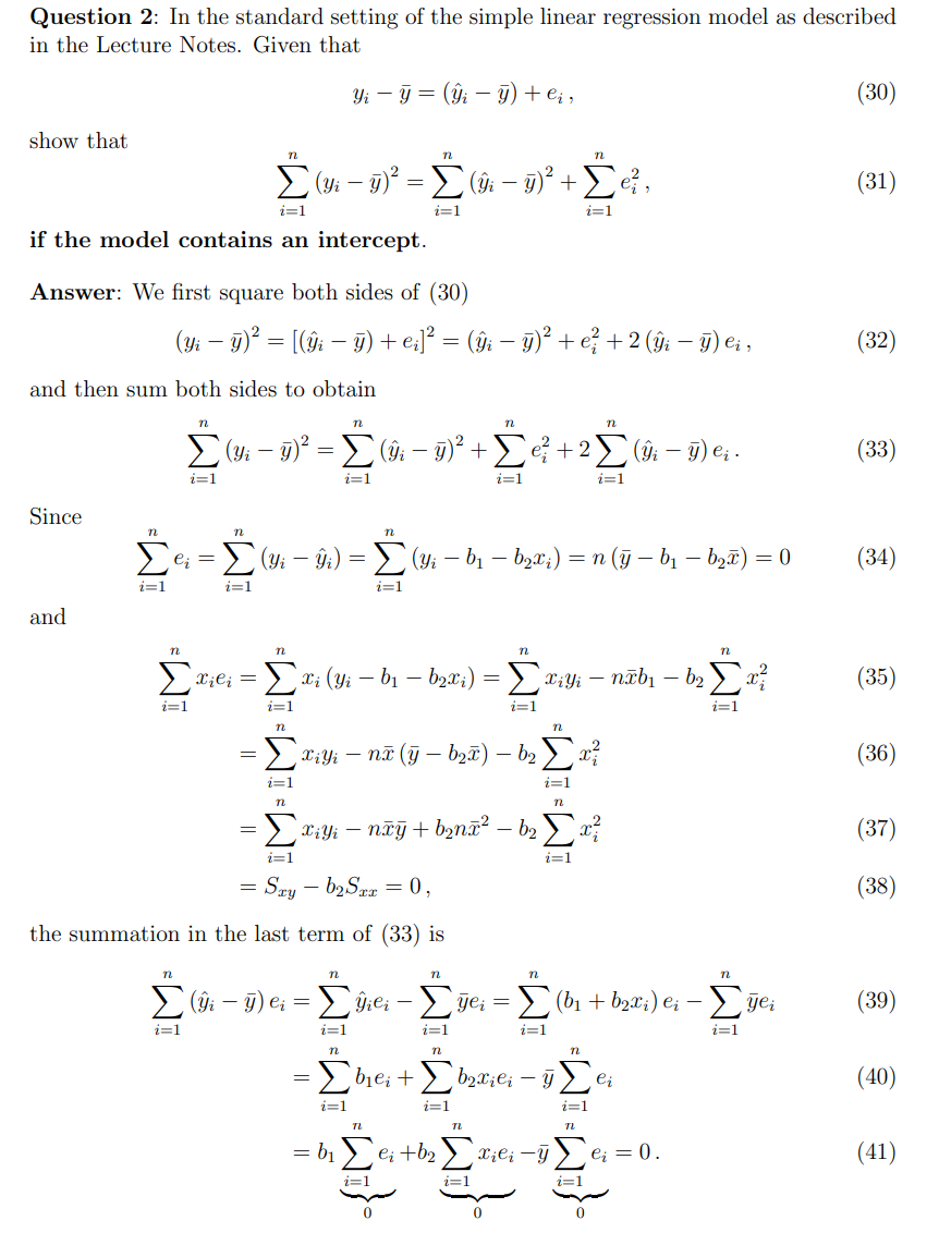
contains an intercept
例题
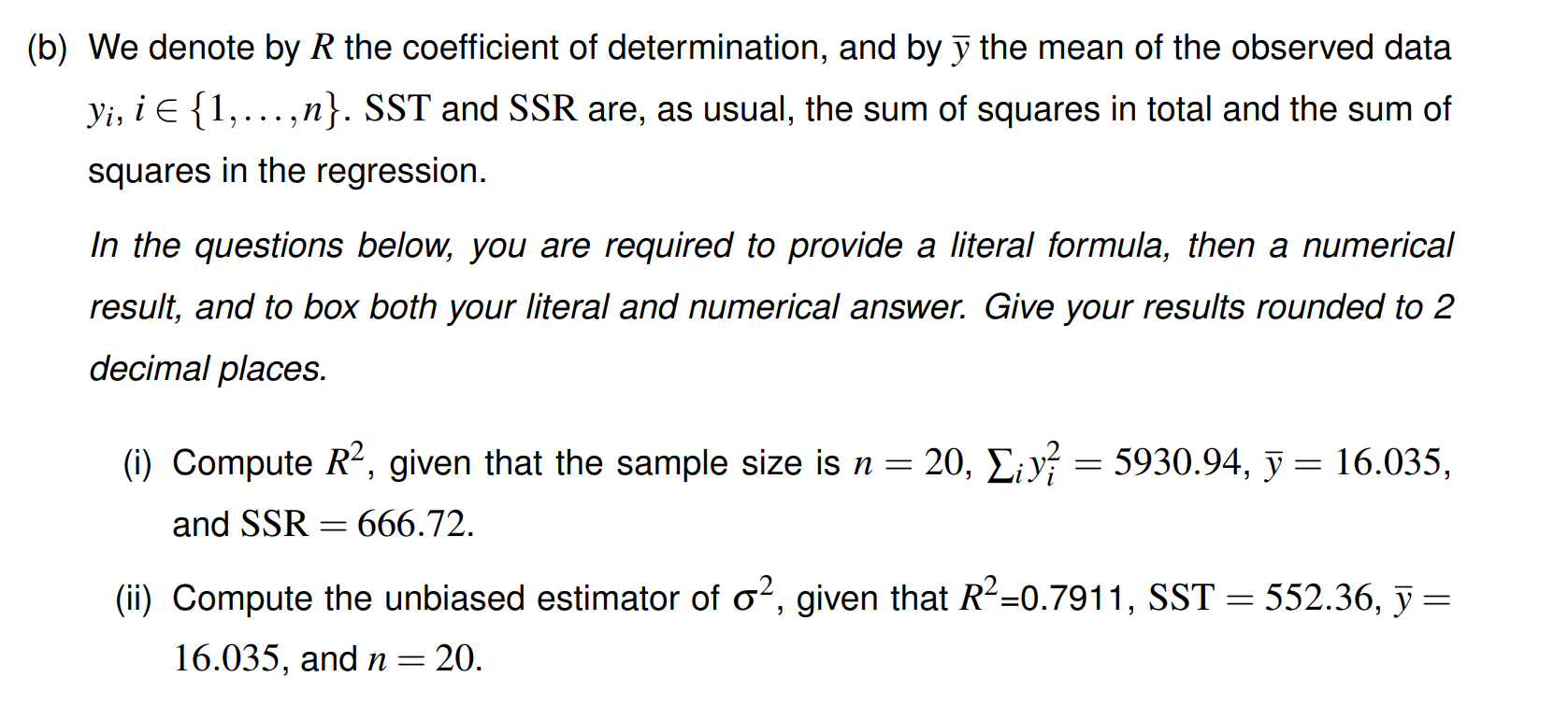
(i) 由
代入数据:
于是
**(ii) **无偏方差估计量为
在本题中
所以
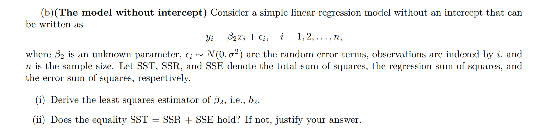
no intercept
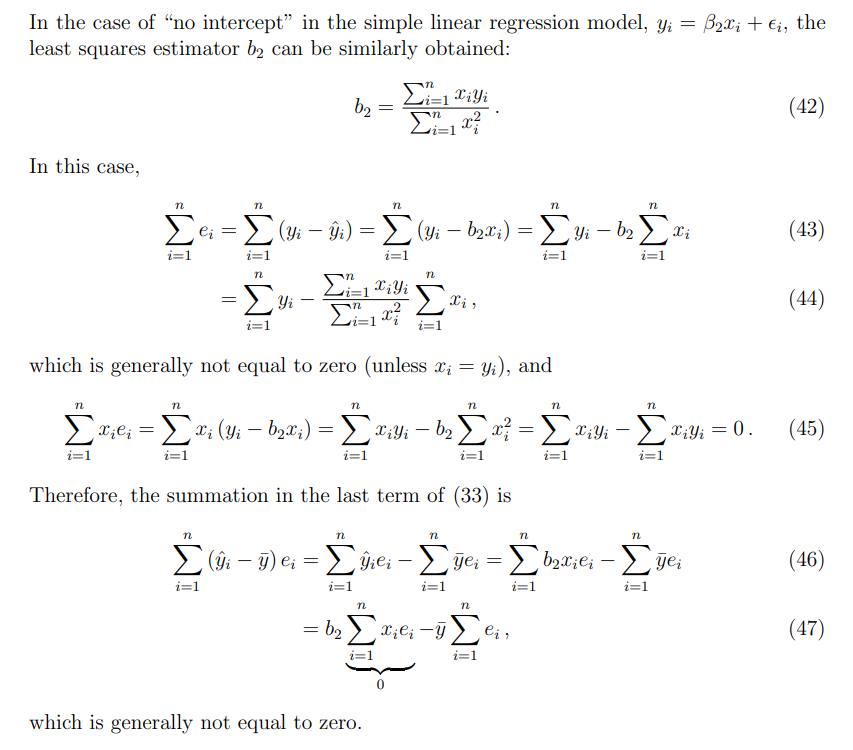
通常线性回归模型有 SST = SSR + SSE,其中 SST 是总平方和。但是这个结论依赖于模型包含截距项,因为截距确保残差均值为 0 并且方差分解成立。
在本题中 没有截距,所以一般 SST ≠ SSR + SSE。等式不成立的原因是残差的正交性条件(残差与拟合值正交)被破坏。
例题
The cross-term $2∑{i}^n(y{i}−\hat{y_{i}})(\hat{y_{i}}−\bar{y})
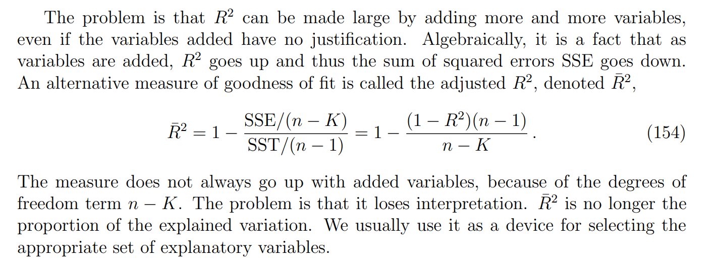
Adjusted
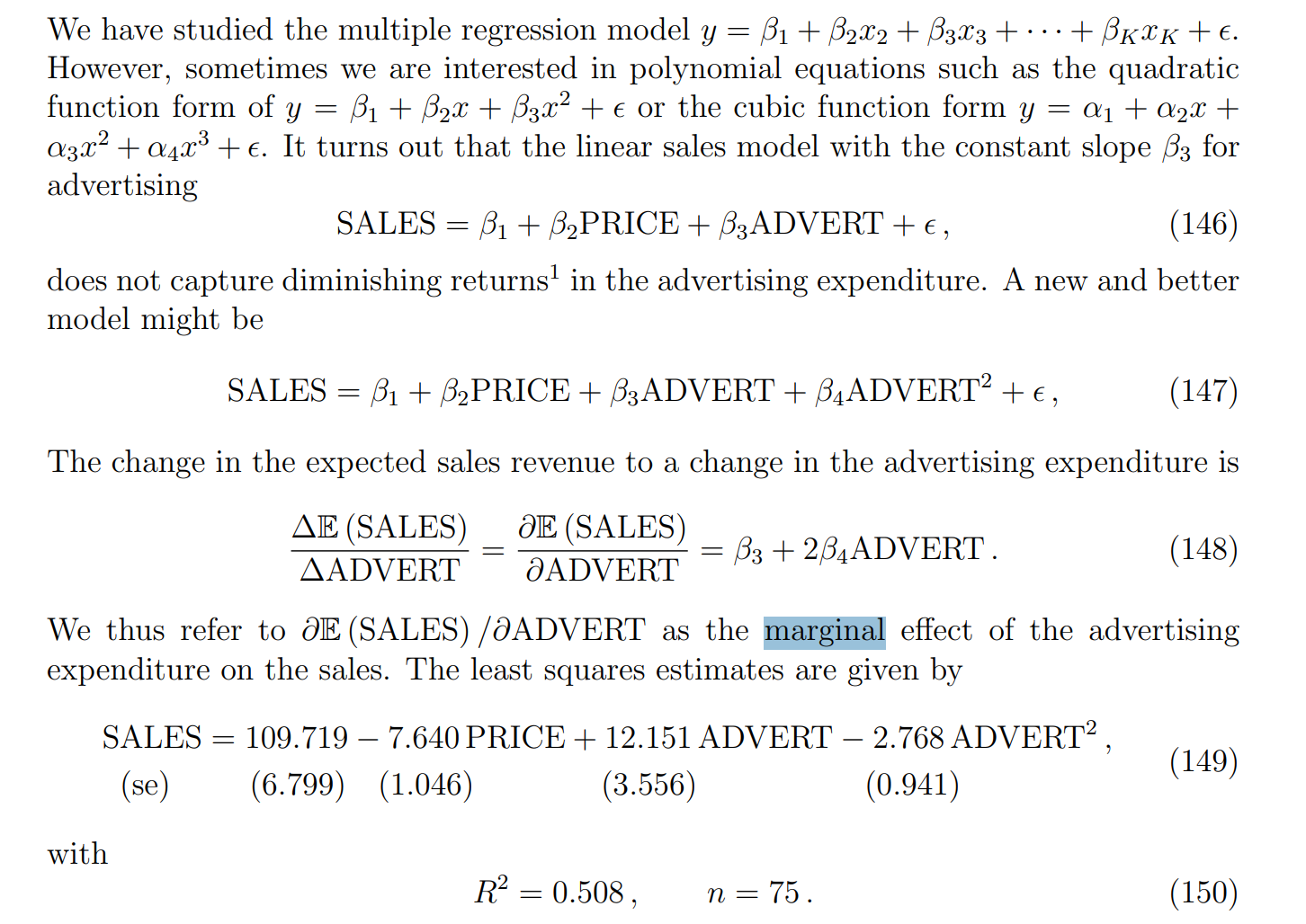
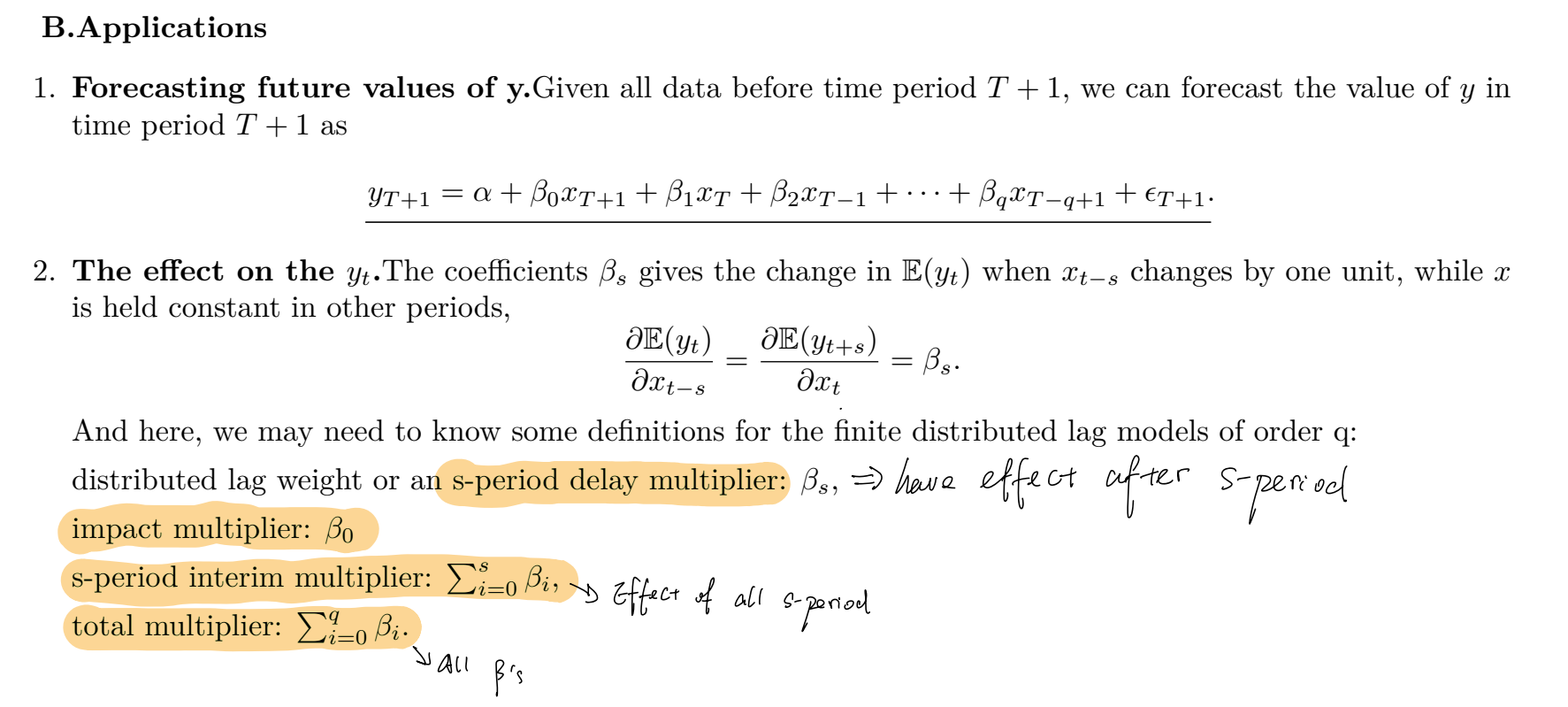
Marginal effect
Chow test(思想)
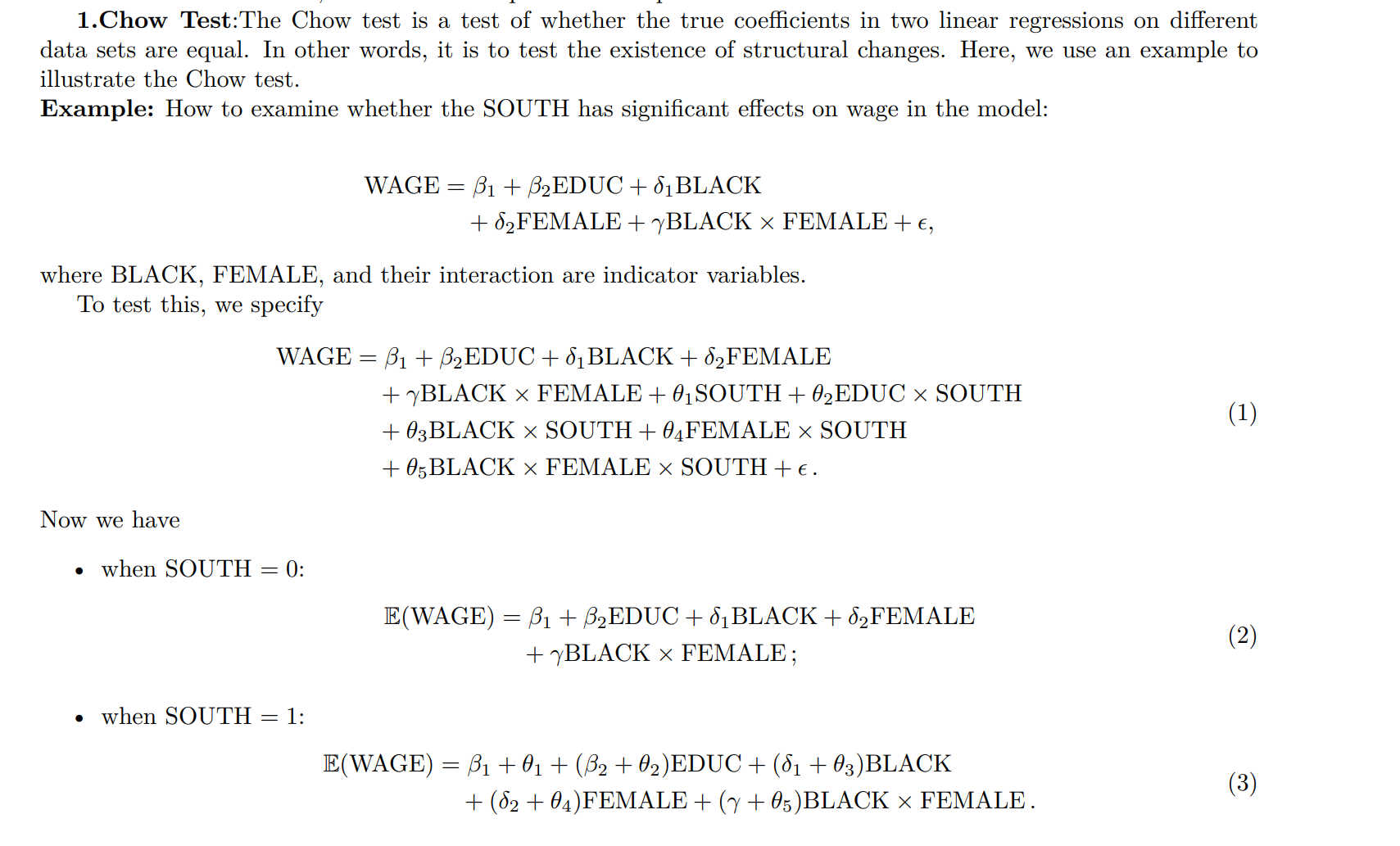
Chow test 可以理解为“通过构造时间 dummy 变量及其交互项来检验结构变化
例题
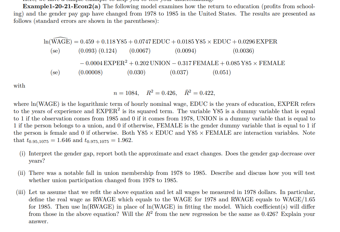
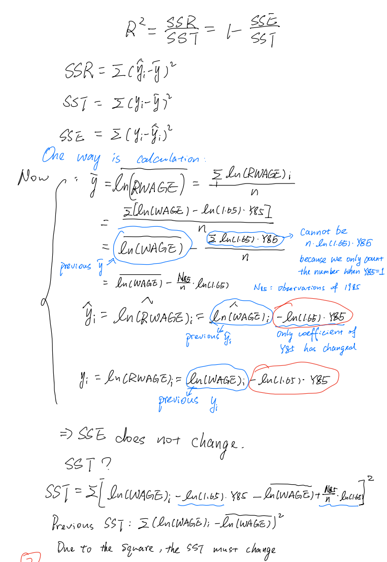
Log-linear models
Exact interpretation
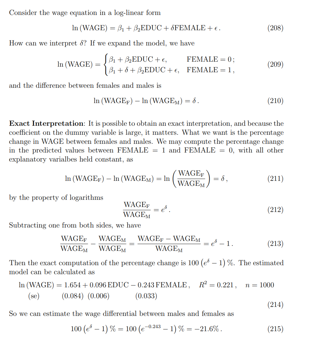
注意:这里是以男性male为基准组。
必须满足两个条件同时为真:
FEMALE 只出现一次(线性项)
FEMALE 不与任何变量交互
只要满足这两点,男女工资差永远是 β₈,不会涉及其他 β。
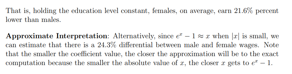
在这个回归里,因为 FEMALE=1,男性是基准,所以标准解释是「女性比男性少 21.6%」。
这里最关键的问题是 “差异是相对谁来衡量”。
一般定义
当我们说 A 比 B 少 x%,数学上意思是:
也就是说:
分子:差值(A − B)
分母:基准组(B)
百分比差异:相对基准来衡量。
代入工资例子
假设表述是:
“Female earn 20% lower than Male.”
这里的基准是 Male,所以式子是:
也就是说:女性工资比男性工资低 20%。
如果表述是:
“Male earn 25% more than Female.”
基准变成了 Female,所以式子是:
Alternative hypothesis
模型中女性虚拟变量是:
其中
FEMALE = 1 → 女性
FEMALE = 0 → 男性
因此:
所以:
当
:女性工资低于男性 当
:男女工资相同 当
:女性工资更高
Approximate Interpretation
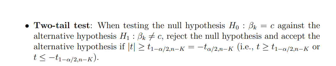
T-test
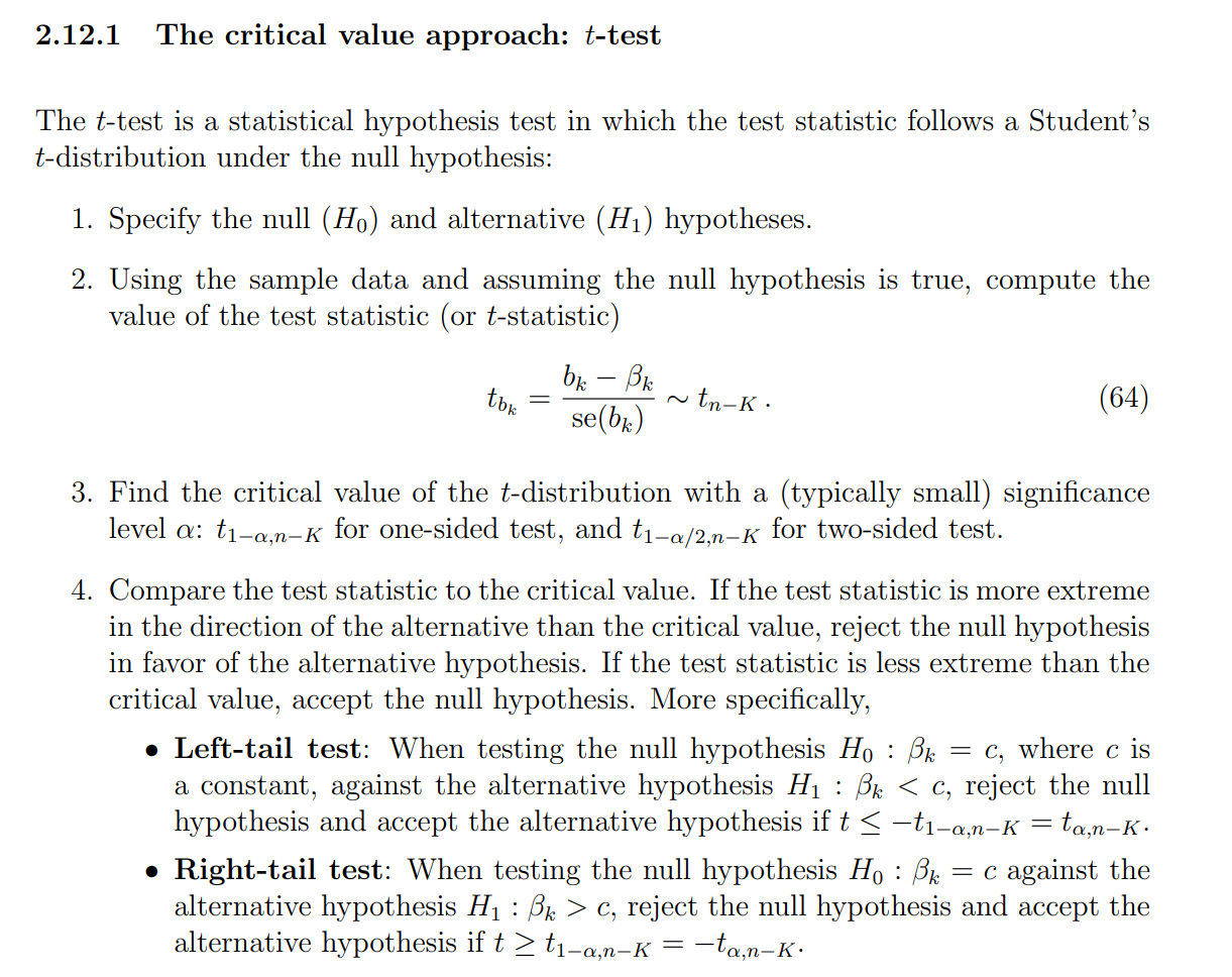
t 值越“大”(绝对值越大),代表系数越显著;但“越大越好”只在检验显著性这一点上成立,不代表模型整体就好
用 test statistic 的方法时,你先算出样本的 t 值,然后在 t 分布图上把它当作横坐标,再与给定显著性水平 α 对应的**临界值
而用 p-value 的方法时,本质上是把观测到的 t 值在 t 分布上对应的尾部面积算出来(单侧是一侧面积,双侧是两侧面积之和),然后将这个面积与 α 比较,若
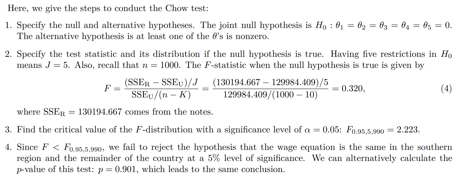
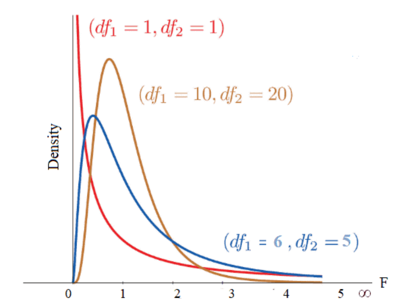
The F-test : joint hypothesis(双边检测看HA)
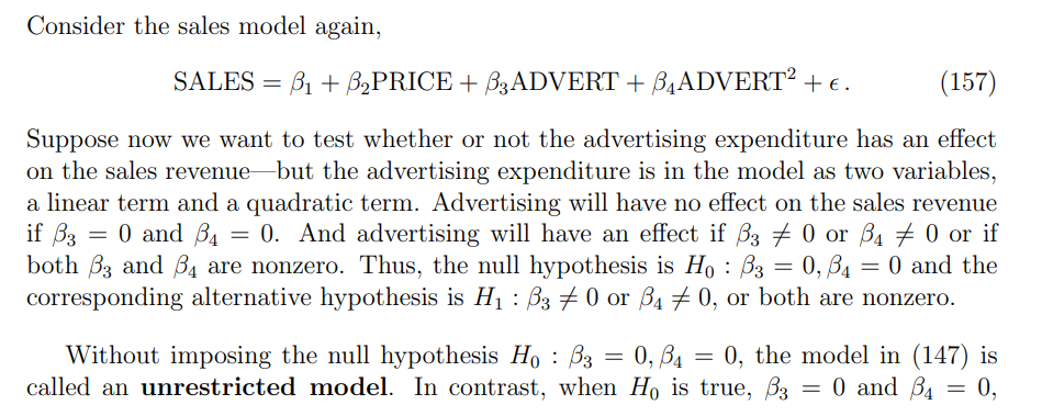
注意:让
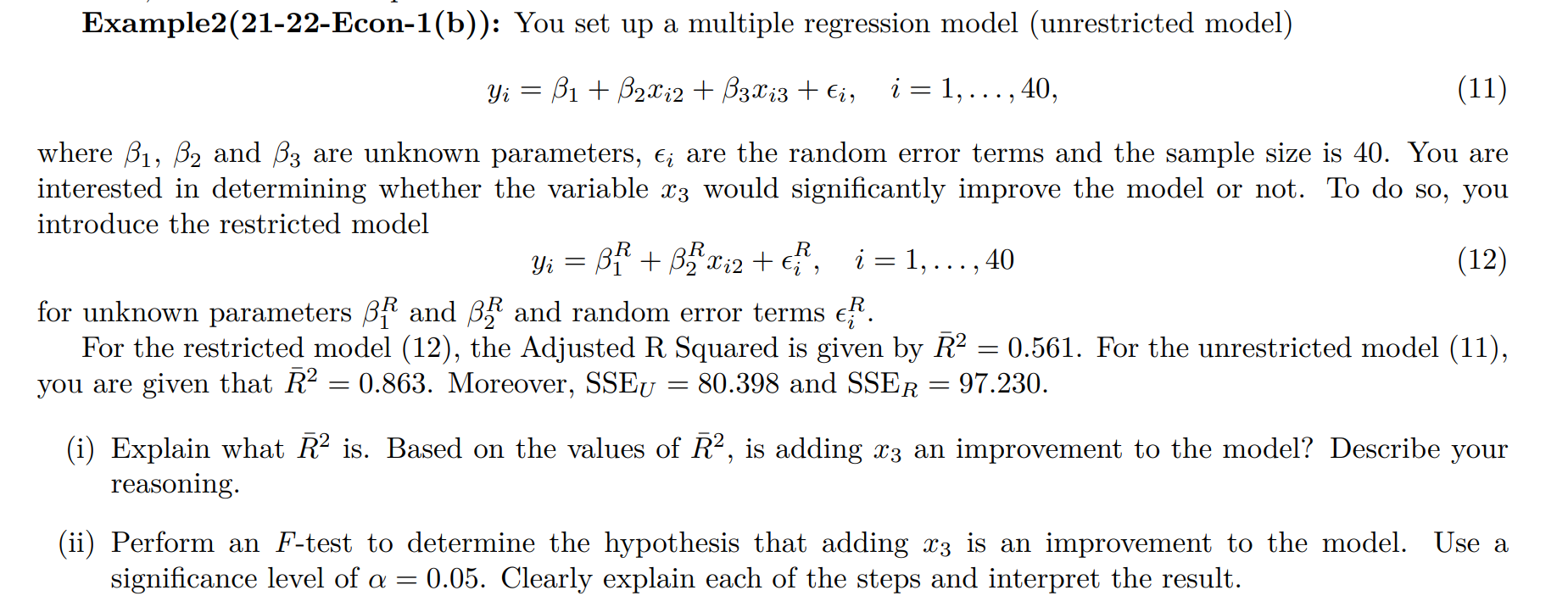
(i)
(ii)注意题目的K还是看回Unstriction model,而且是右侧检验。
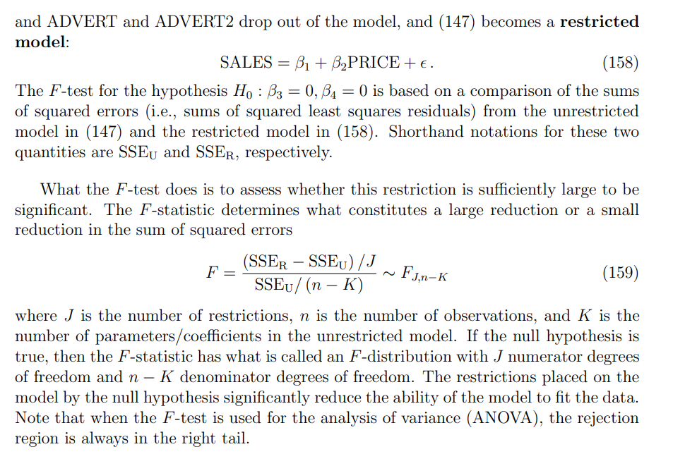
F-test :
注意:这种情况是只剩截距的
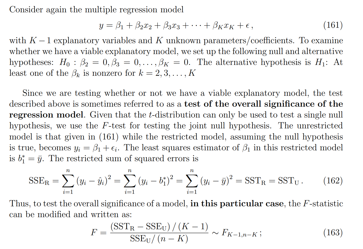
这里的推导流程是:要把
这个量 SST只依赖于观测数据本身(样本数量 n 和样本值
例题
考点常规
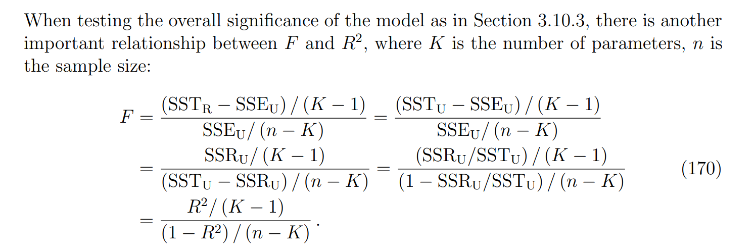
利用F=t^2
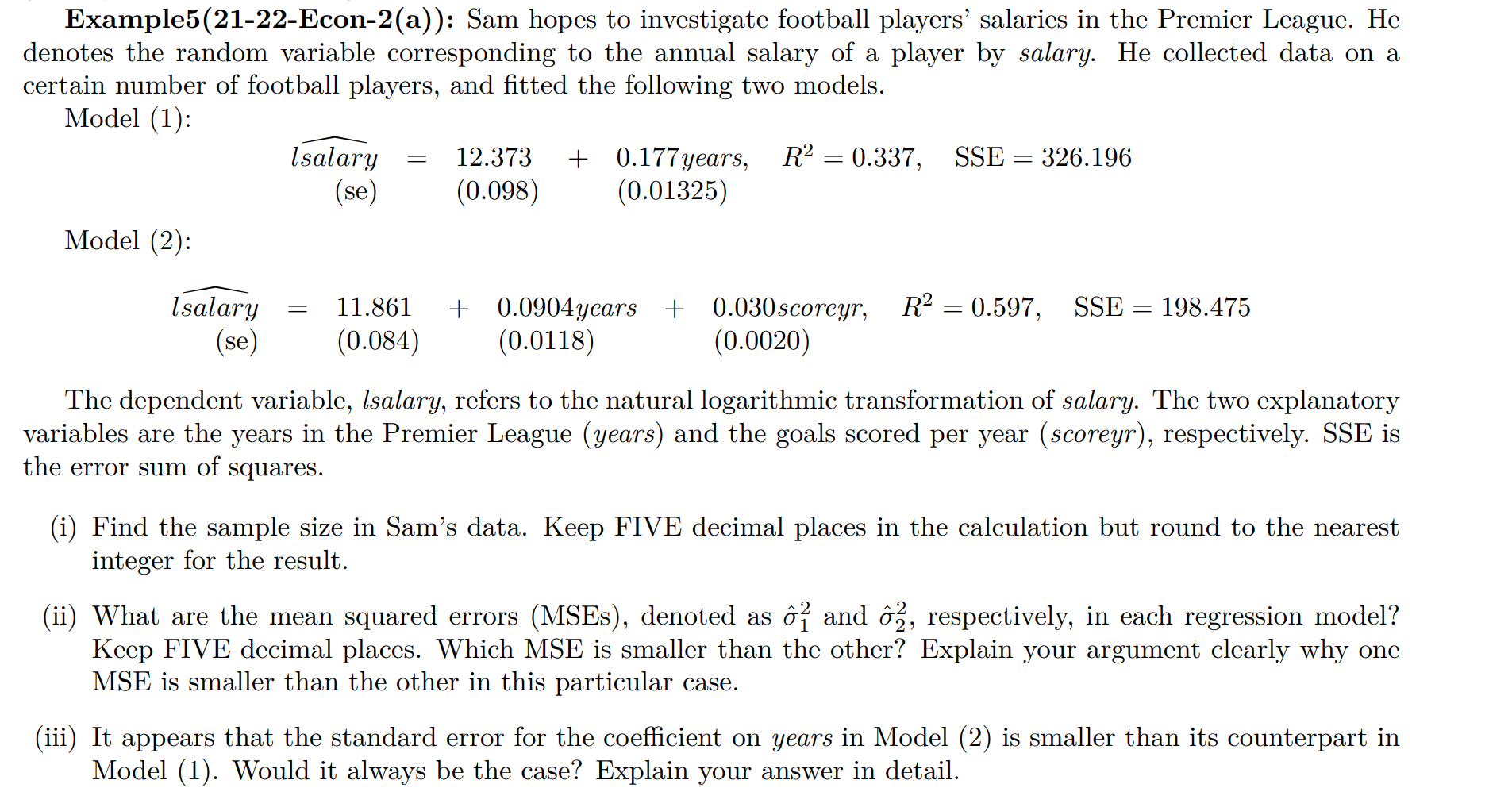
注意这里求出t的时候要平方才等于F,而且F是只对model 1 自己用。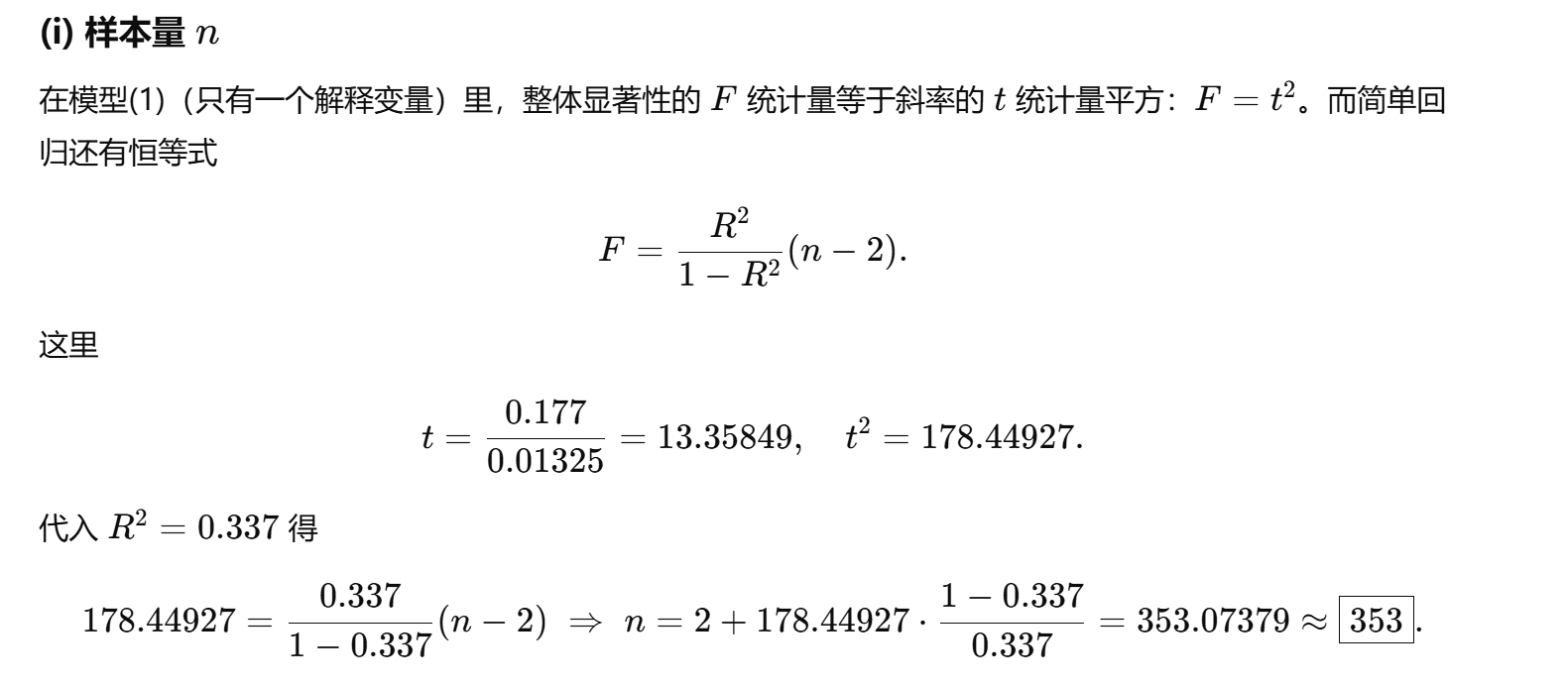
现实中
计量经济学里对
Least square prediction
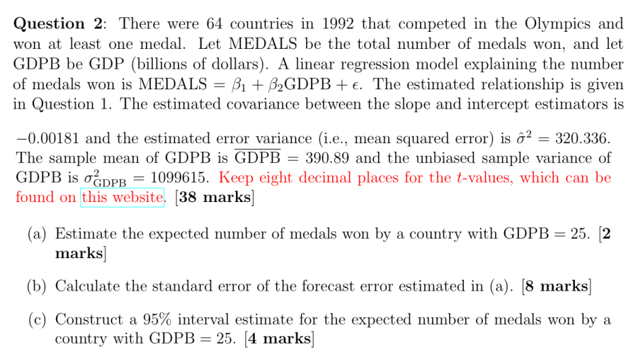
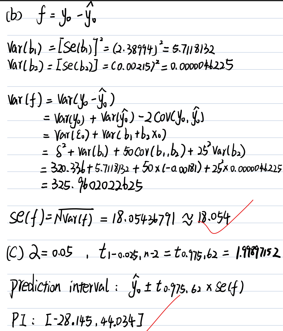
注意这里的prediction interval 和 confidence interval区别:
prediction interval: 预测某一个特定国家的GDP=25的奖牌数
confidence interval:估计所以GDP为25国家的奖牌数
Heteroskedasticity(方差随自变量变化)
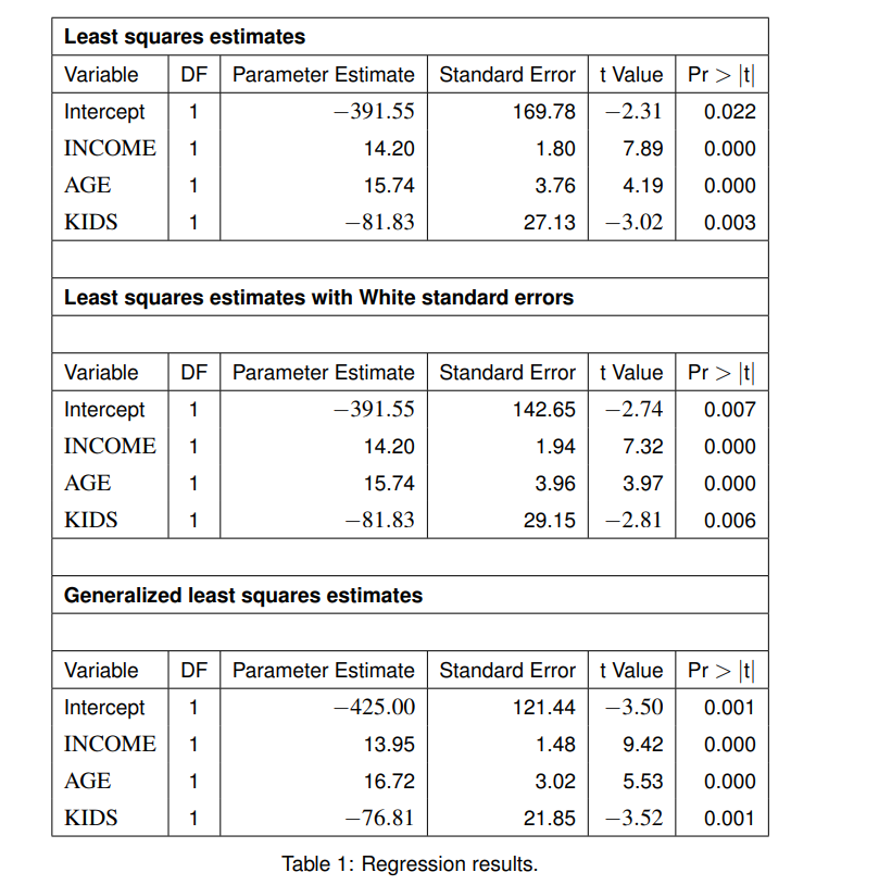
解释 Pr>|t| 的意义”
Pr>|t| = 在系数其实等于 0 的假设下,我们仍然观察到如此极端 t 值的概率。
→ 小,则强烈证明系数不是 0。
→ 因此变量对 MILES 有显著影响。
The Goldfeld–Quandt test(双边检测看HA)
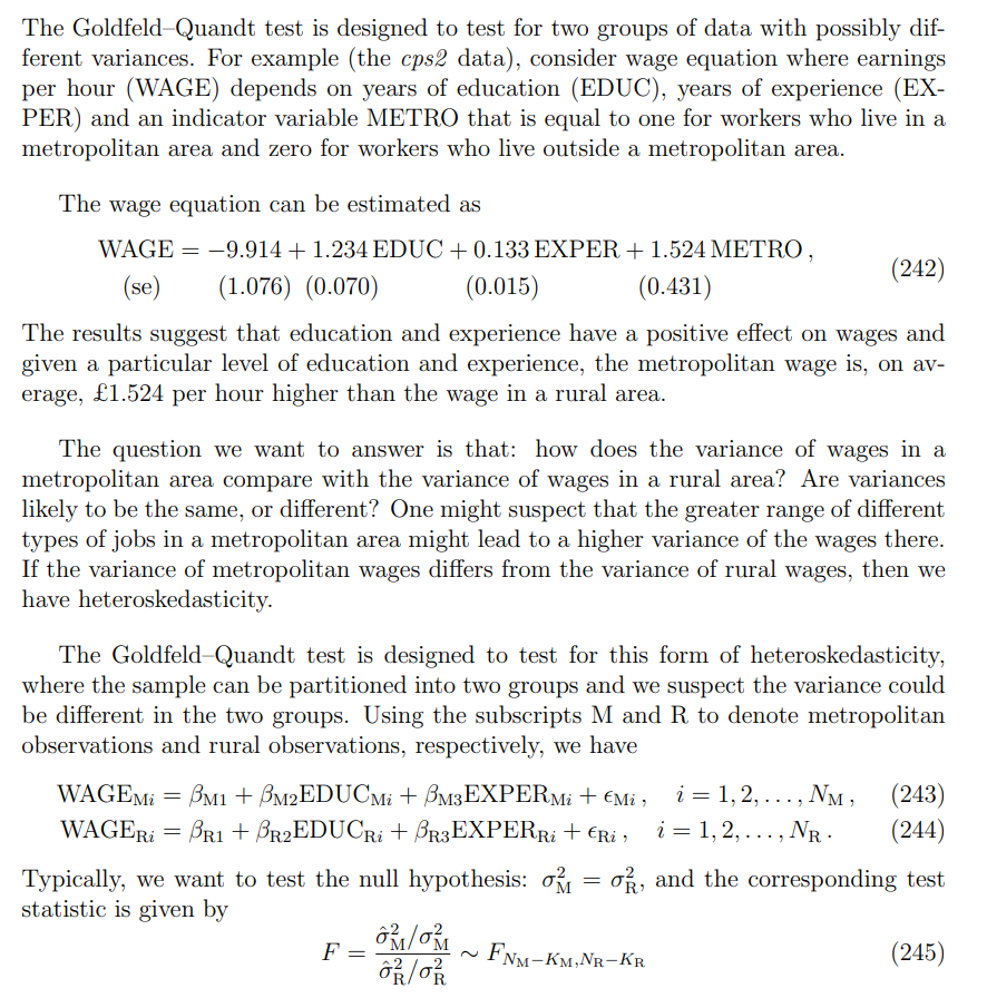
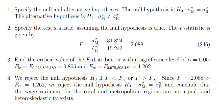
当题目已经给出说分成两组数据的时候使用。
例题:
题目要求
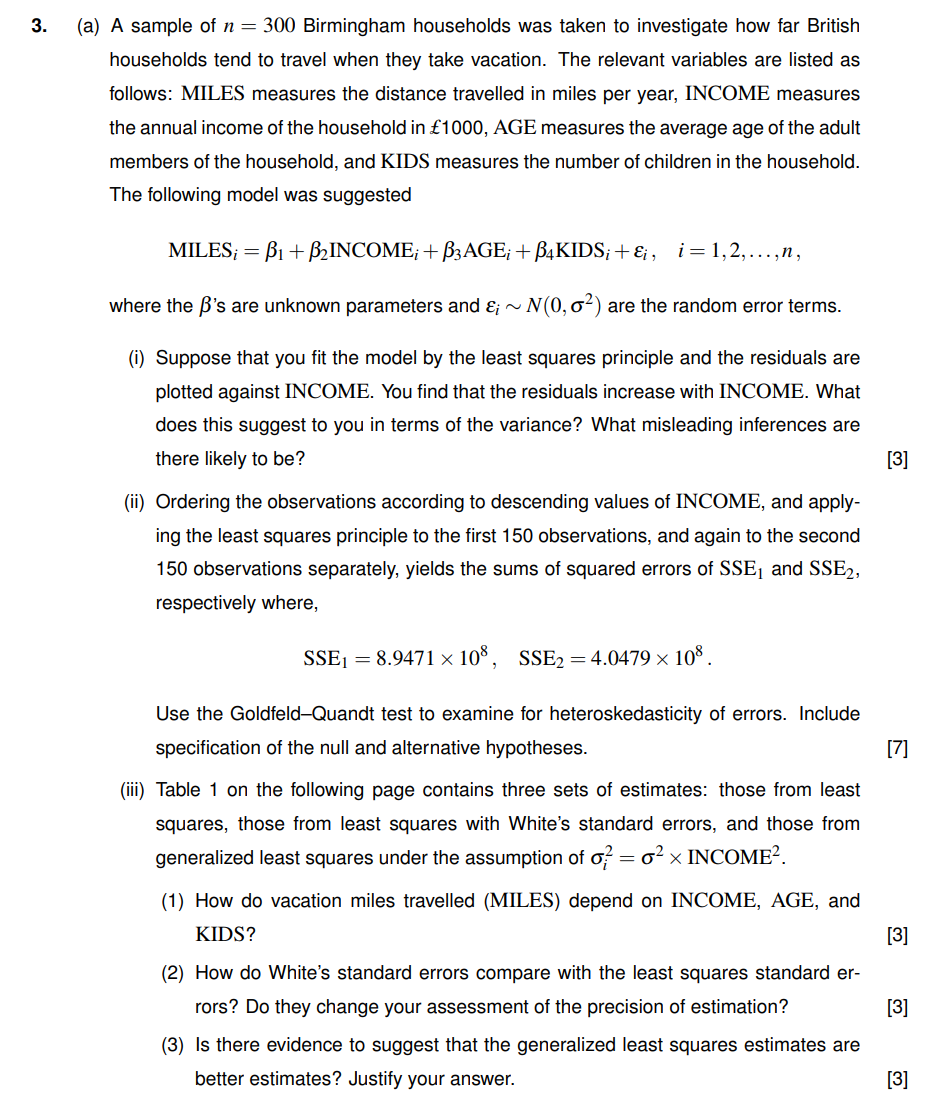
分成两组考点
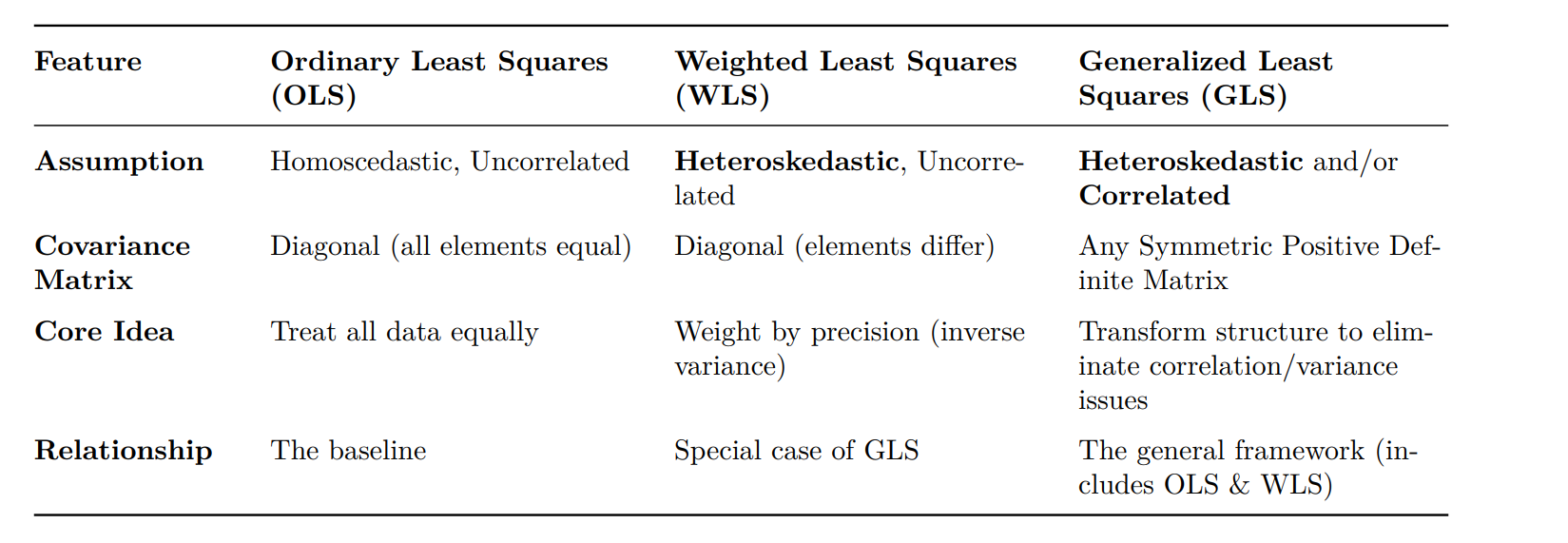
OLS WLS GLS
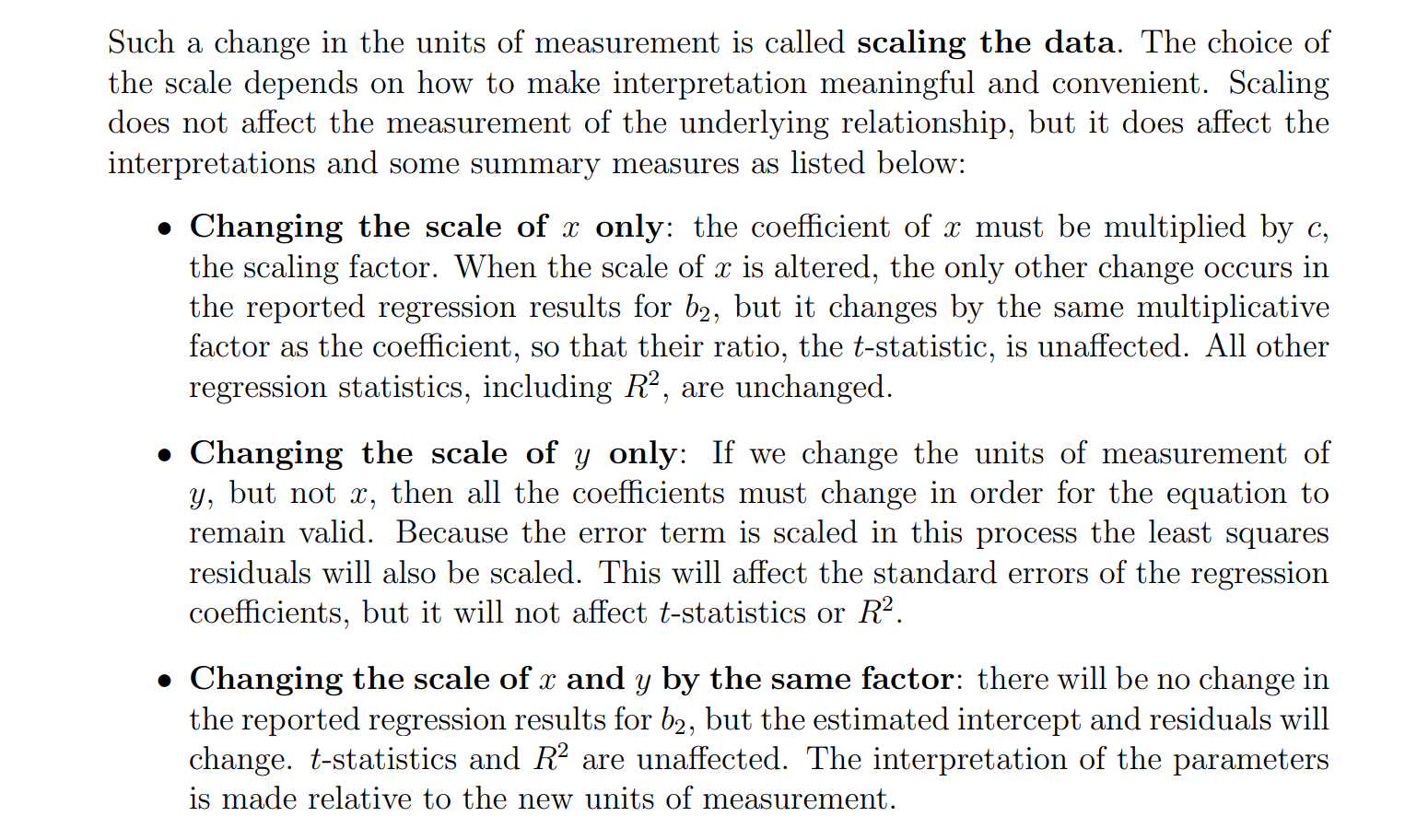
Scaling the data
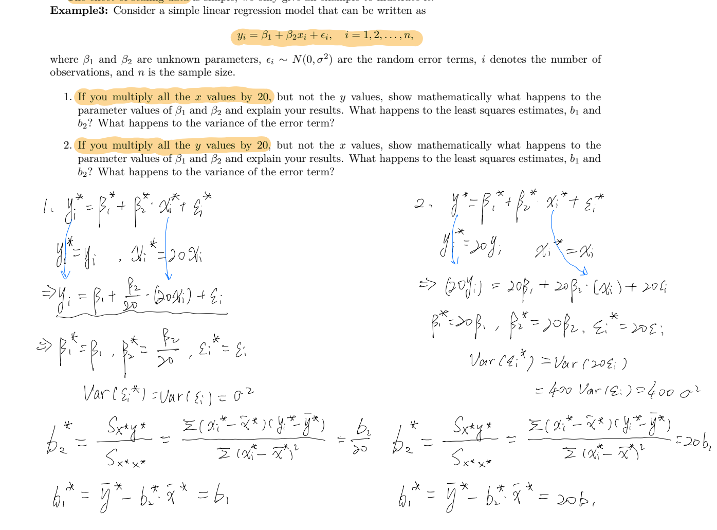
例题:
Elasticity
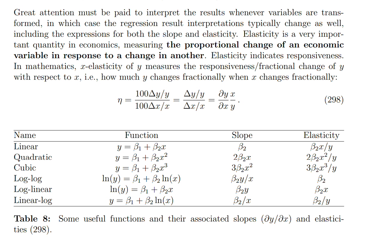
链式求导:
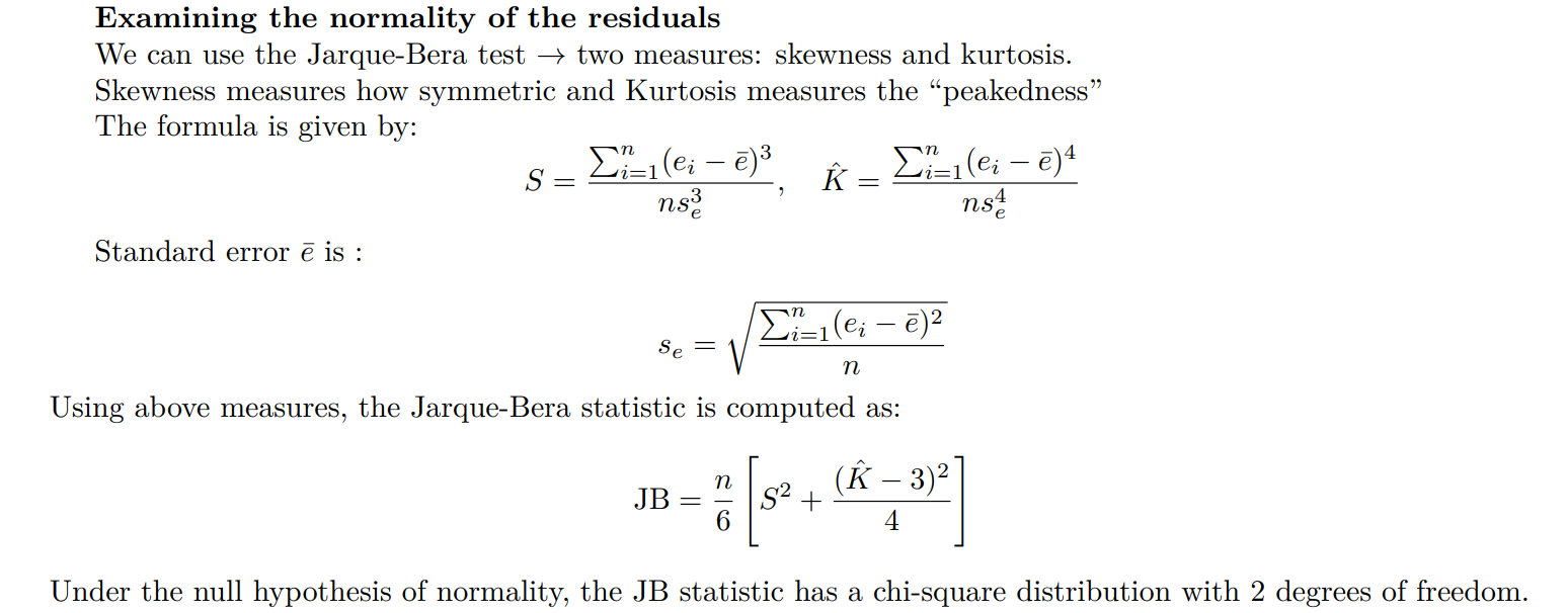
Jarque-Bera test(skewness kurtosis)检测是否 normality
例题(原始峰度:Kurtosis>=1)
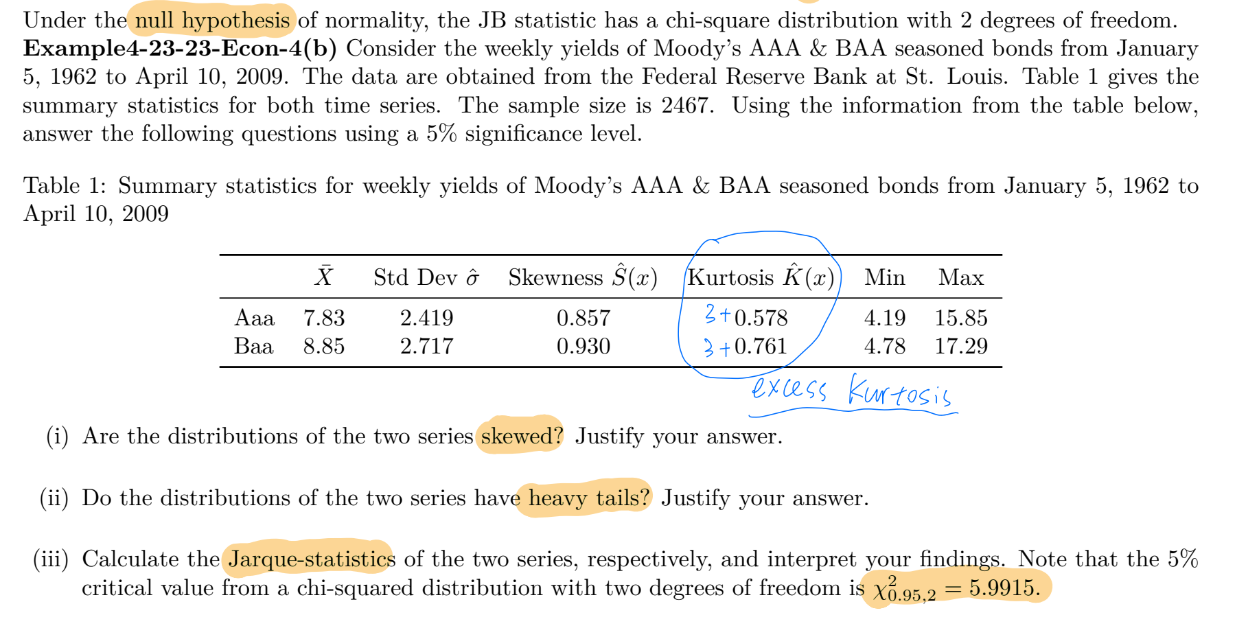
(i) Are the distributions of the two series skewed? Justify your answer.
Yes, both distributions are skewed. The sample skewness for the AAA series is 0.857, and for the BAA series it is 0.930. Both values are positive. A positive skewness indicates that the distribution has a longer right tail, meaning the mean is greater than the median, and the distribution is right-skewed (positively skewed).
(ii) Do the distributions of the two series have heavy tails? Justify your answer.
Yes, both distributions have heavy tails (leptokurtosis). The table reports excess kurtosis (kurtosis minus 3). For the AAA series, the excess kurtosis is 0.578; for the BAA series, it is 0.761. Positive excess kurtosis indicates that the distributions have fatter tails than a normal distribution, meaning extreme values are more likely.
(iii) Calculate the Jarque-statistics of the two series, respectively, and interpret your findings.
The Jarque-Bera (JB) test statistic is used to test whether the series follows a normal distribution. It is calculated as:
where n is the sample size, S is the sample skewness, and K-3 is the sample excess kurtosis. The sample size is n = 2467. At the 5% significance level, the critical value from the chi-squared distribution with 2 degrees of freedom is
For the AAA series:
- Skewness ( S = 0.857 )
- Excess kurtosis ( K-3 = 0.578 )
For the BAA series:
- Skewness ( S = 0.930 )
- Excess kurtosis ( K-3 = 0.761 )
Interpretation:
Both JB statistics (AAA ≈ 336.26, BAA ≈ 415.14) are much larger than the critical value of 5.9915. Therefore, we reject the null hypothesis of normality at the 5% significance level for both series. This indicates that the distributions of AAA and BAA bond yields are significantly non-normal, consistent with the observed positive skewness and positive excess kurtosis.
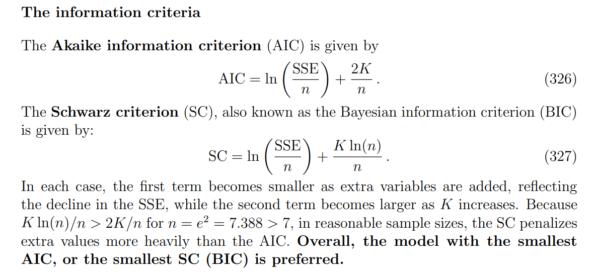
AIC and SC(负责做模型选择,在“拟合得好”和“模型别太复杂”之间做权衡)
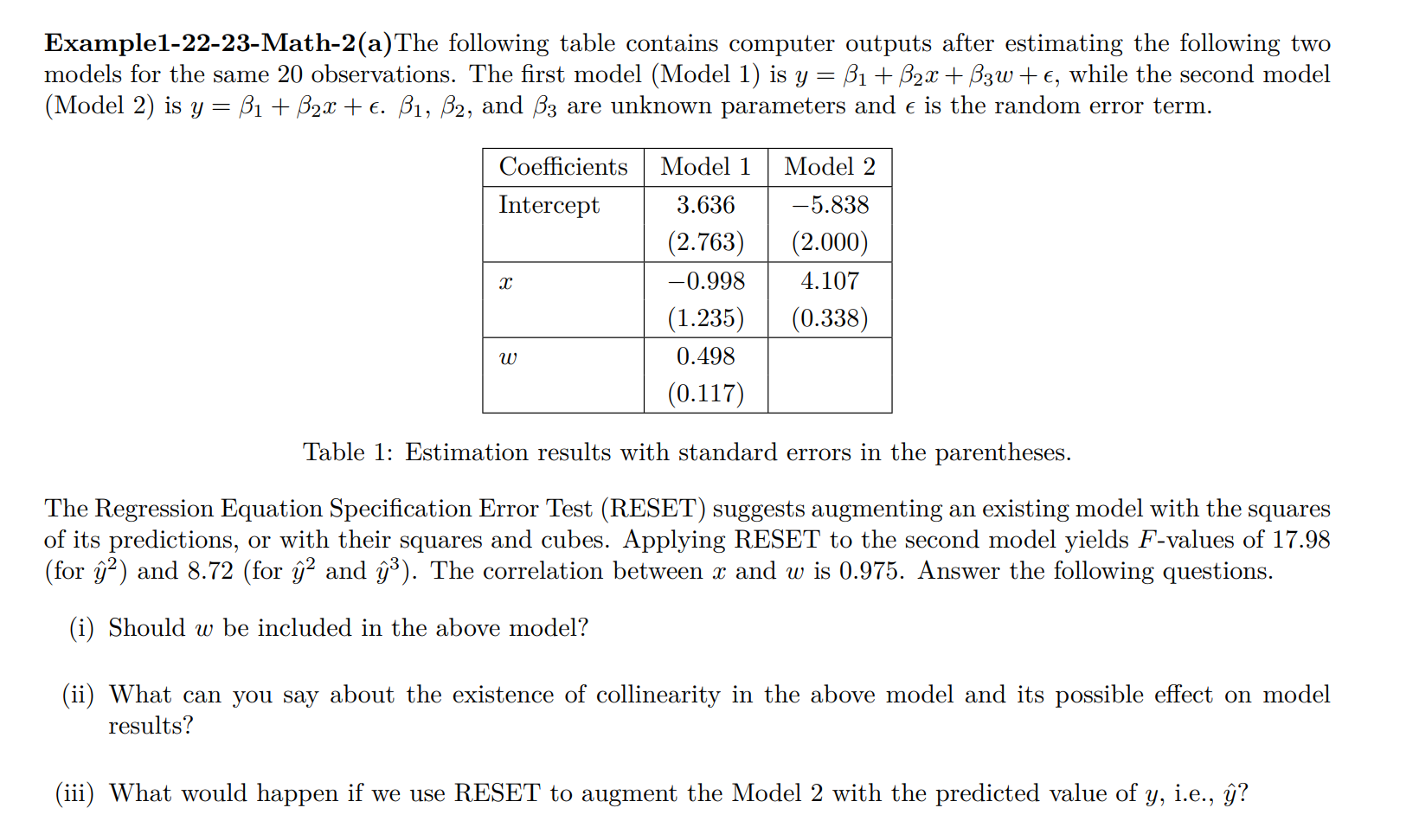
RESET(先估计原始线性模型,得到拟合值
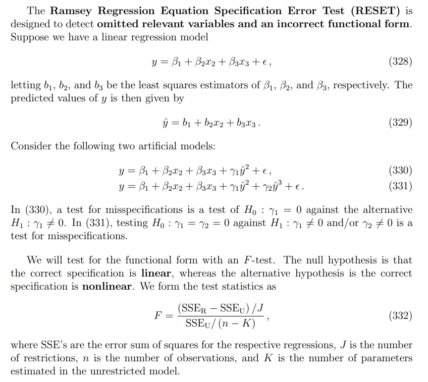
注意:一般拒绝就是说忽略了重要的变量没有加入。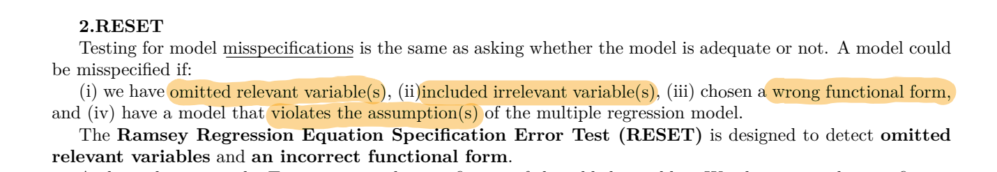
缺点:
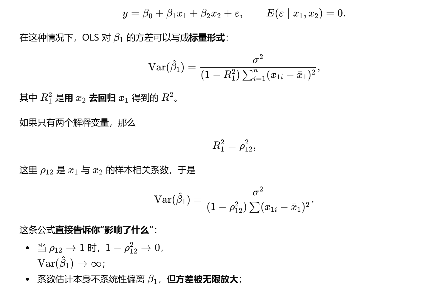
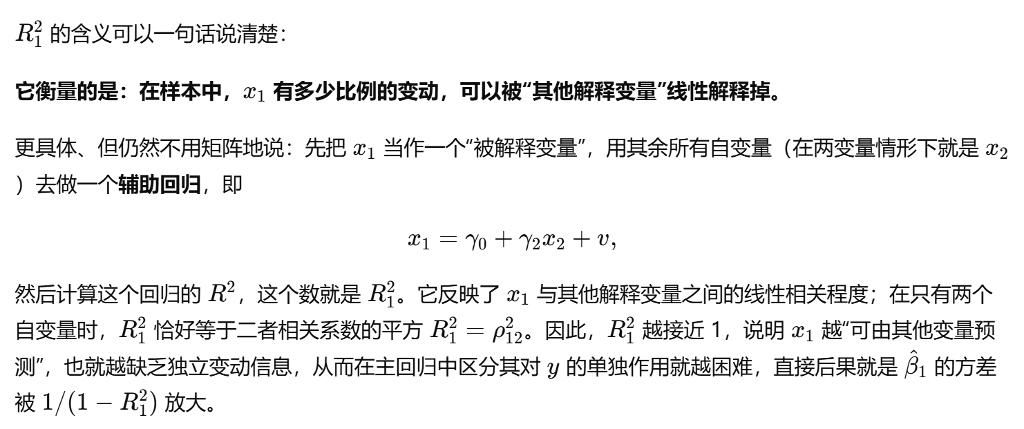
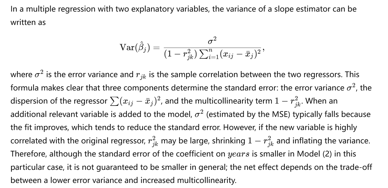
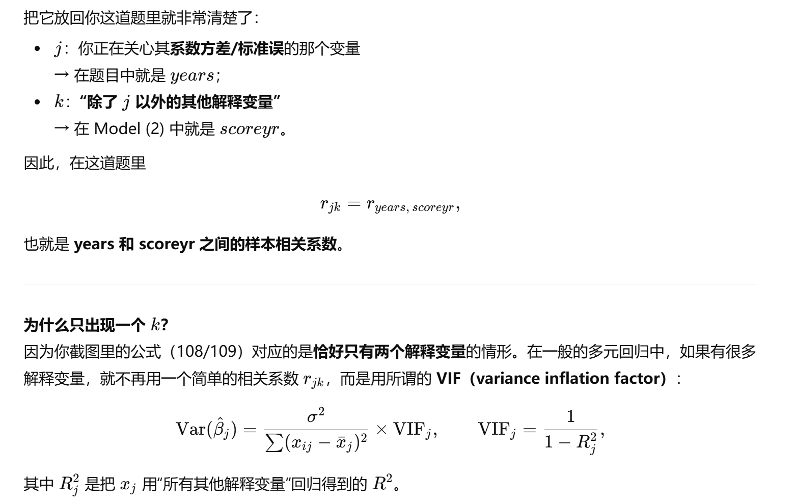
collinearity
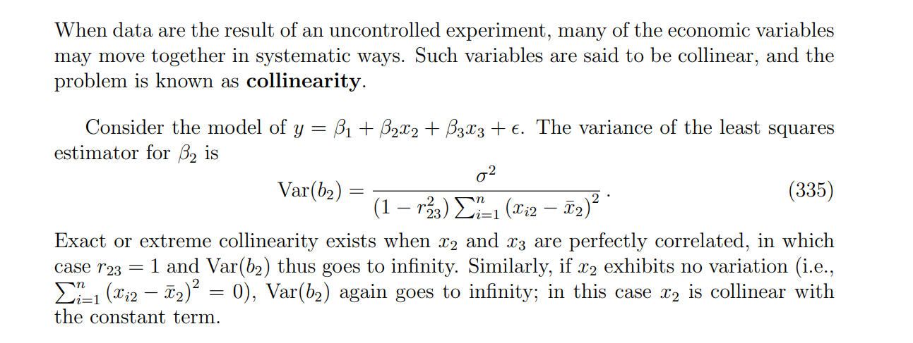
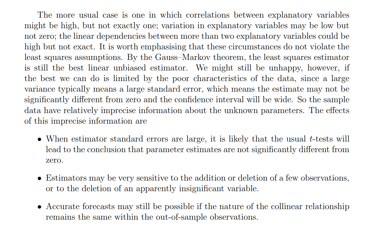
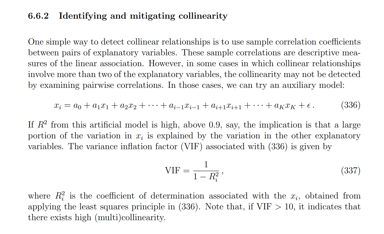
注意看 correlation coefficient ,加入参数然后标准差是否变大,系数符号是否翻转。
例题
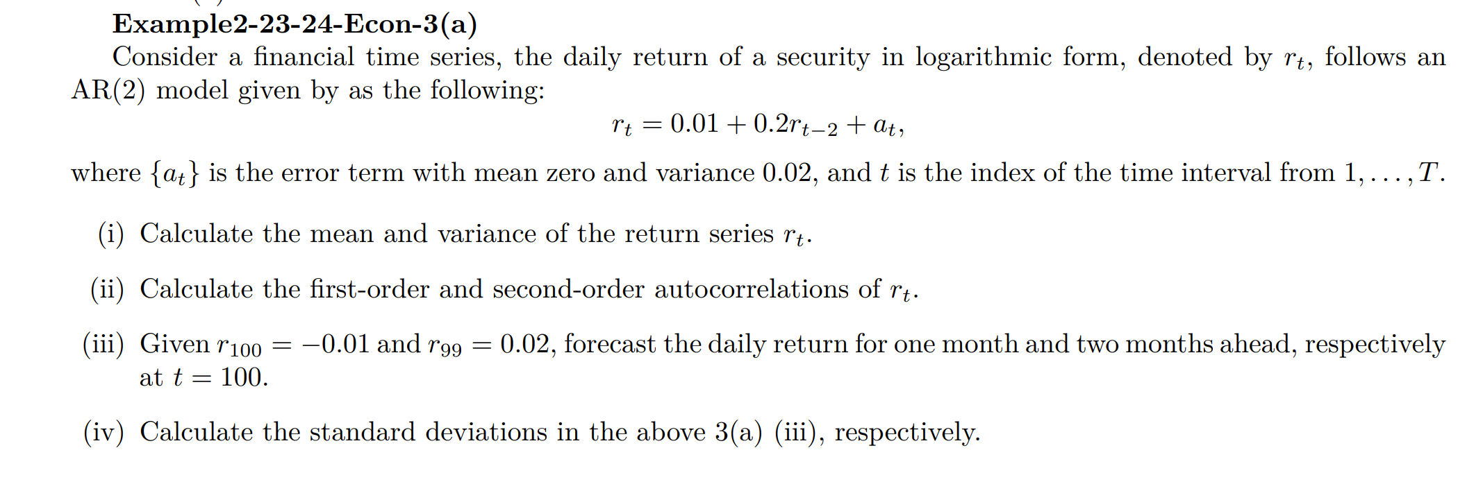
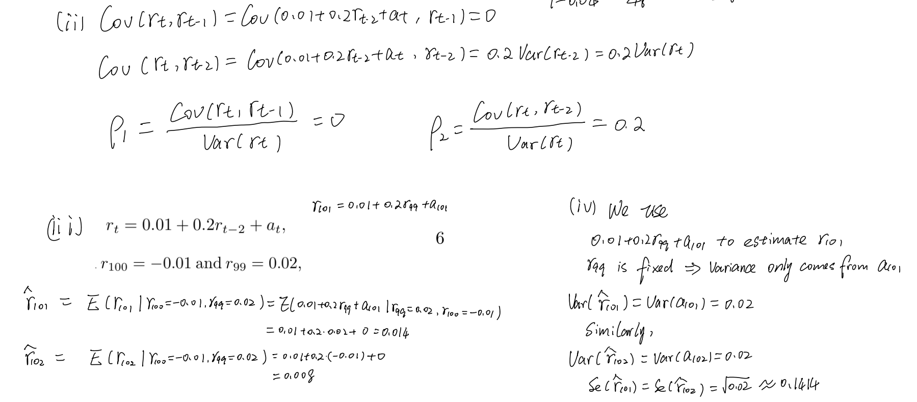
Stationarity
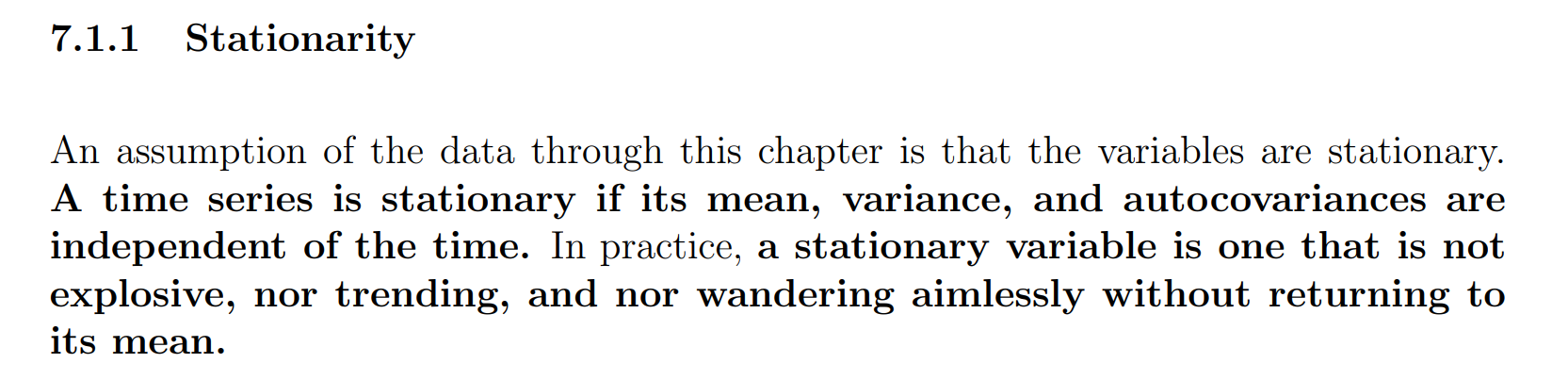
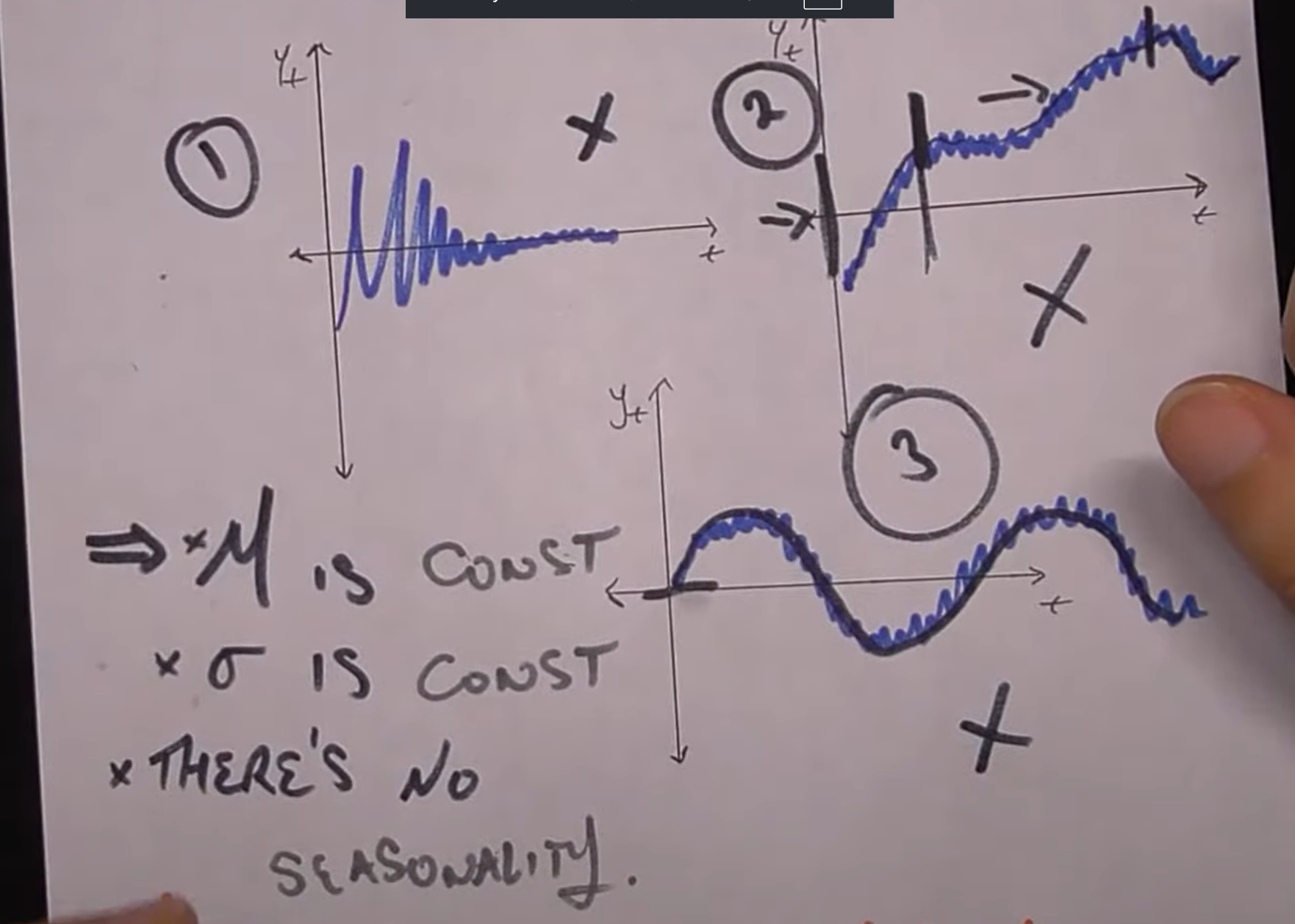
Time series(所谓的“预测”指的就是条件期望(conditional expectation))
例题
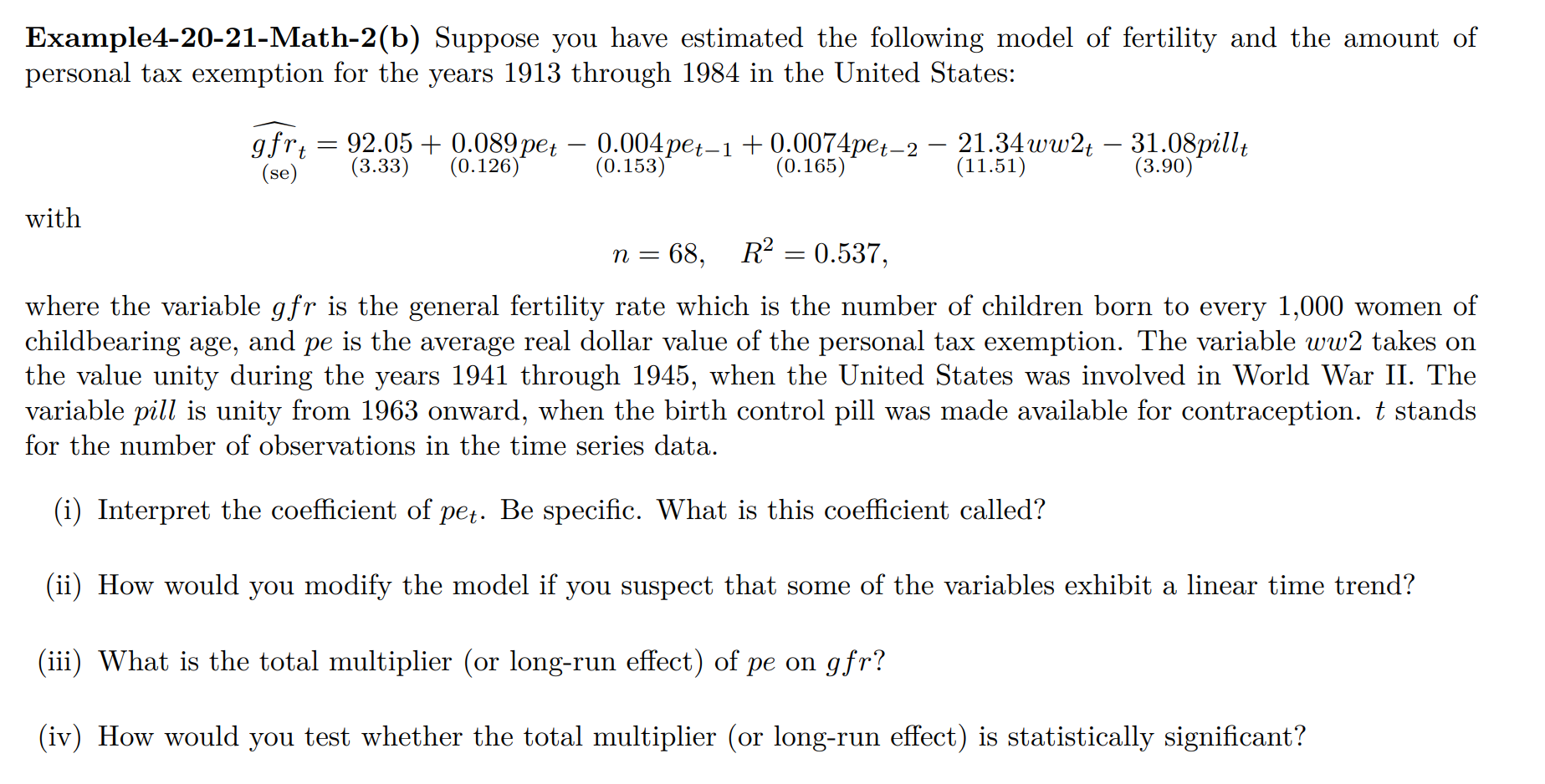
(ii) 如果怀疑变量存在线性时间趋势,应如何修改模型?
若怀疑 gfr、pe 等变量随时间呈现系统性的线性趋势,应在回归中 加入时间趋势项,即在模型右侧加入 (t):
这样做的目的,是将生育率和税收政策可能共同受到的长期趋势(如社会结构变化、长期经济发展)从估计中剥离,避免由于 遗漏趋势变量 而导致 (pe) 系数的伪相关或偏误。
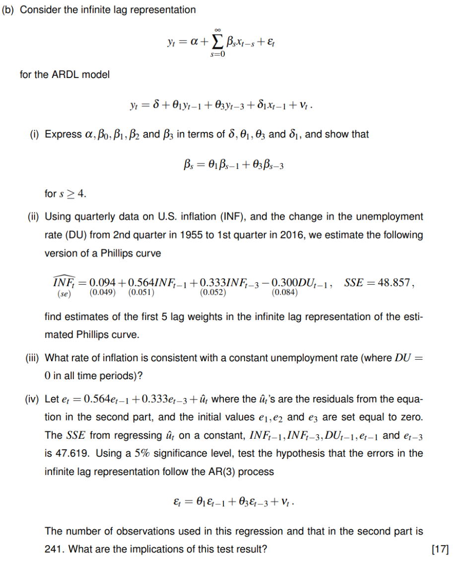
(iv) 如何检验该 total multiplier 是否显著?
要检验长期效应是否显著,本质上是在检验如下线性假设:
F 检验:将上述线性约束直接写成一个线性限制,对联合假设进行检验;
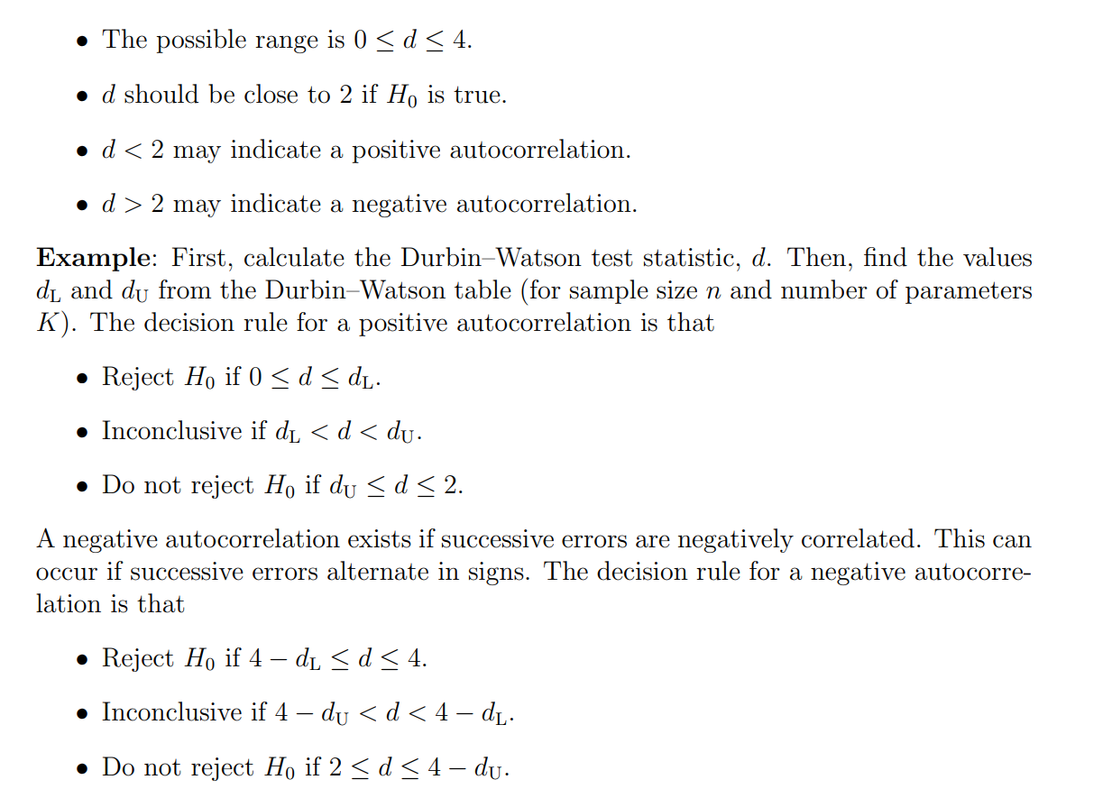
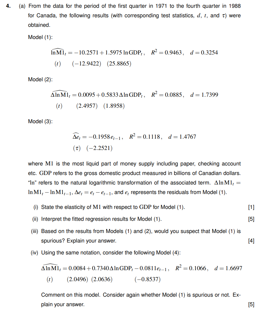
Durbin-Watson Test(残差相关性)
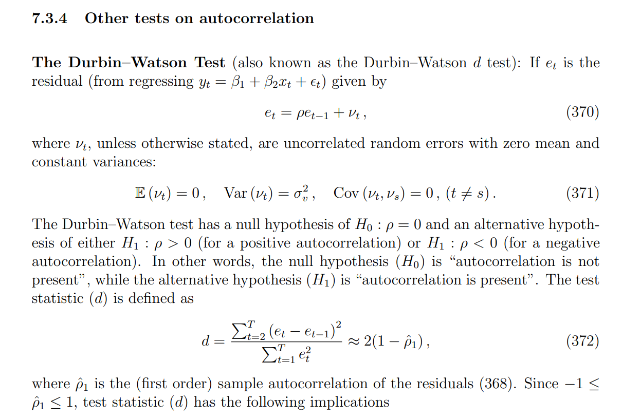
注意:
例题
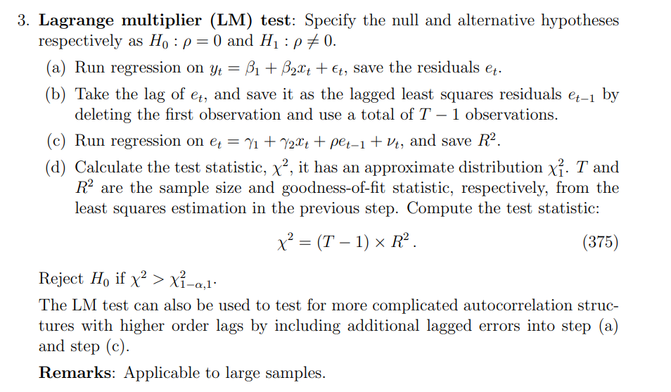
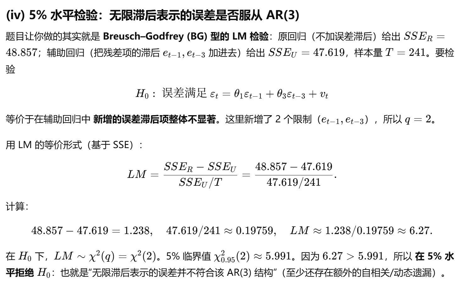
LM test
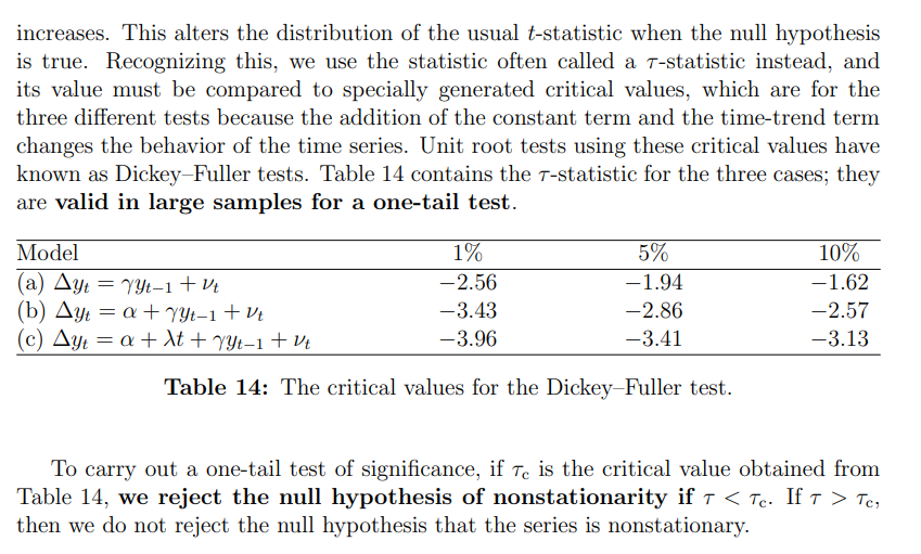
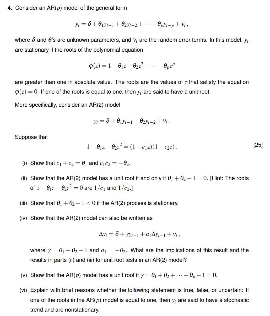
Dickey–Fuller test(单边,是否yt平稳ADF,默认epsilon平稳)
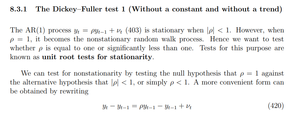
注意:等于1不平稳,是随机游走
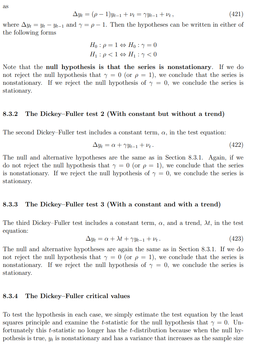
注意:
拒绝
例题
random walk
AR model:(默认:由白噪声驱动的)
ECM
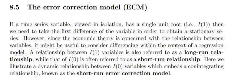

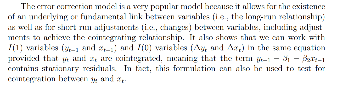
| 名称 | 是什么 |
|---|---|
| ECT | |
| ECM |
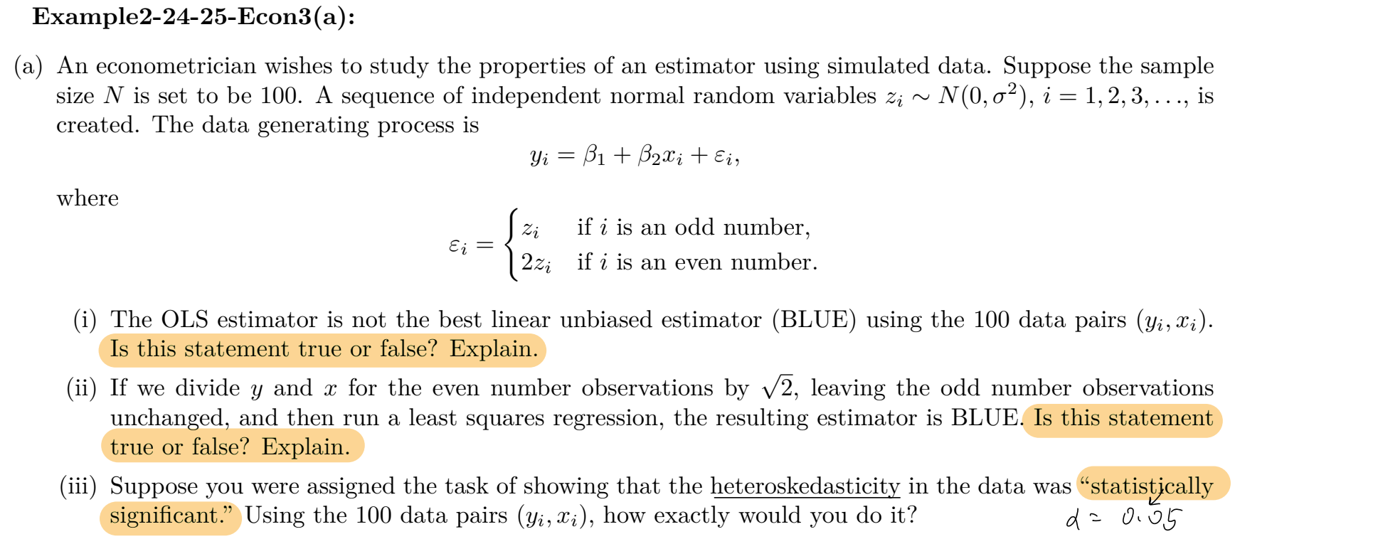
判断题
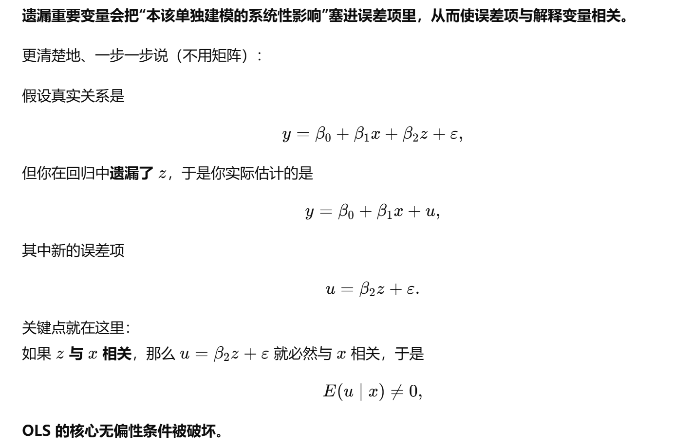
估计变量有偏
是的,无偏性的核心条件就是在给定解释变量的情况下,误差项 (
这一定义的含义是:在控制了所有解释变量之后,误差项中包含的那些未观测因素不再系统性地与解释变量相关,因此在重复抽样下,正负误差会相互抵消,使得 OLS 估计量的平均值等于真实参数;如果只满足无条件的 (
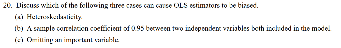
异方差:只影响方差Var(